Gravity and Levity

How can electrons be “topological”?

July 14, 2020

by Brian

The following text is an excerpt from a draft of an article that I co-wrote for the magazine Physics Today, together with Prof. Art Ramirez at UC Santa Cruz. The article will appear (edited, and with more professional figures) in the magazine in September. The article attempts to give some intuition about the concept of “topological” electron bands, which have become very important in modern condensed matter physics.

Dawn of the Topological Age?

Historians often label epochs of human history according to their material technologies. For example, we have the bronze age, the iron age and, more recently, the silicon age. From the physicist’s perspective, the silicon age began with the interplay of theory, experiment, and device prototyping of a new type of material, the semiconductor. Semiconductors had been known since the late 1800s as materials with unusual sensitivity to light, to the method of synthesis, and to the direction of current flow. It was not until the early 1930s, however, that a theoretical understanding of semiconductors approached its modern form [1]. The prevailing view at the time saw metals and insulators as opposite limits of electron itineracy, adiabatically controlled by the probability for an electron to hop between atoms. But the recently-developed idea of accessible electron energies (bands) and inaccessible energies (band gaps) provided a natural category for semiconductors – they were more like insulators, but with smaller band gaps, often controlled by impurities. The next fifteen years witnessed breakthroughs in the purification and control of dopants in the elemental semiconductors silicon and germanium that eventually enabled the discovery of transistor action at Bell Labs in 1947. A surprise came during the transistor patent preparation, however. The basic idea underlying the field effect transistor had already been patented in 1930 by Julius Lillienfeld, an Austrian-Hungarian physicist who had emigrated the United States in 1921.

For semiconductors, the path from materials discovery to device implementation was neither linear nor easily predicted. For a relatively new class of materials, called “topological” materials, one can notice compelling analogies with the development of semiconductors, suggesting the tantalizing possibility that we are at the dawn of the “topological age”. In this article, we will describe what it means for materials to be “topological,” and why topology raises the prospect for revolutionary new devices.

The “shape” of an electron band

The notion of a topological invariant comes from a branch of mathematics called topology, which studies properties of geometric objects that are conserved under continuous deformations. The most famous such property is the genus, g, which is an integer that counts the number of holes in a three-dimensional (3D) shape (i.e., g = 0 for a sphere or a plate, g = 1 for a donut or a coffee mug, g = 3 for a pretzel, etc.). The genus is defined via the Gauss-Bonnet theorem, which states that the integral of Gaussian curvature K over the surface S of an object is quantized:

$\frac{1}{2 \pi} \int_S K dA = n$

Here $n$ is an integer that is related to the genus by $n = 2(1-g)$ . For example, for a sphere with radius $R$ , the curvature $K = 1/R^2$ is a uniform constant, so the integral over the surface area gives $n = 2$ , which is consistent with the genus $g = 0$ of an object that has no holes in it. The remarkable implication of the Gauss-Bonnet theorem is that, if one stretches the sphere in any arbitrary way, so that some parts of the surface become more curved and other parts become flatter, the integer n remains unchanged. The integrated curvature is invariant (see Fig. 1).

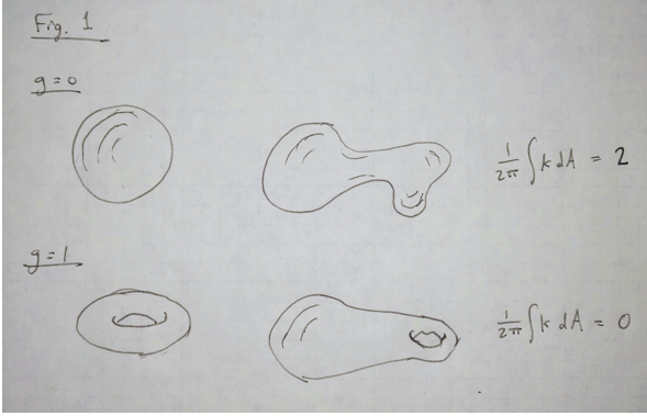
Fig. 1 A topological invariant is a property of a geometric shape that does not change when the shape is stretched or distorted. One such invariant is the genus g, which is defined by the number of holes in the surface and is related to the integral of the Gaussian curvature K over the surface of the shape. For example, shapes with no holes in them (g = 0) all give the same value of this integral, as do shapes with one hole in them (g = 1).

Much of the recent excitement surrounding “topological electronics” originates in the prospect of finding physical properties of electronic systems that behave like this integer-valued genus. Such an invariant property is necessarily robust to small perturbations or defects, since integers cannot change continuously. In the remainder of this section we will explain the origin of a commonly-discussed invariant, the Chern number, which is what defines a “topological electron band”.

Within a single isolated atom, electrons occupy discrete quantum energy levels, or orbitals. When many atoms are arranged into a crystal, the wave functions from neighboring atoms hybridize with each other, and the orbitals broaden into bands of states having a range of energies. Each of the states within a band describes an electron that is shared among many atoms, and its wave function can be written in terms of the momentum $\vec{p}$ with which the electron hops from one atom to another:

$\psi_{\vec{p}}(\vec{r}) = u_{\vec{p}}(\vec{r}) e^{i \vec{p} \cdot \vec{r}/\hbar}$ .

The factor $e^{i \vec{p} \cdot \vec{r}/\hbar}$ in this wave function resembles the usual “plane wave” state that describes free electrons. But this plane wave is multiplied by a function $u_{\vec{p}}(\vec{r})$ , called the “Bloch function” (after Felix Bloch [3]), that repeats periodically for each identical unit (the unit cell) of the crystal and describes the way that the electron is affected by atomic nuclei within the unit cell. As we will see, it is the Bloch function that contains information about the topology of the electron band.

Importantly, the electron momentum $\vec{p}$ can take only certain restricted values. Since $\vec{p}$ describes the process of hopping between neighboring crystal lattice sites, the de Broglie wavelength $\lambda = 2 \pi \hbar/p$ associated with the wave function cannot be shorter than the distance between neighboring unit cells of the crystal. Thus, in a given direction, the momentum has a maximum possible magnitude. The space of allowable momenta is called the Brillouin zone, and its shape depends on the arrangement of atoms in the crystal. In discussing the “topology” of an electron band, the Brillouin zone plays the role of a “geometric space”, and closed surfaces within the Brillouin zone are akin to geometric shapes, which can have an integer-valued index akin to the genus. Importantly, exactly opposite points on the zone boundary are equivalent to each other, since they correspond to the same standing wave state with minimal de Broglie wavelength (effectively, the Brillouin zone has periodic boundary conditions).

Constructing an analogy with the Gauss-Bonnet theorem for electron bands requires an analog of the “curvature” that is integrated over a closed surface. As it turns out, this analog of curvature arises from the properties of the Bloch functions $u_{\vec{p}}(\vec{r})$ . To see the analogy, consider asking the question: for a given momentum $\vec{p}$ , where within the unit cell is the electron wave function centered? The usual way to answer this question is to calculate the expectation value of the position operator $\hat{x}$ within the unit cell. Written in terms of momentum, the position operator is $\hat{x} = -i \hbar \nabla_{\vec{p}}$ , and one can write its expectation value as

$\vec{X}(\vec{p}) = -i \hbar \langle u_{\vec{p}} | \nabla_{\vec{p}} | u_{\vec{p}} \rangle$ .

This quantity $\vec{X}$ is called the “Berry connection”, and it can be thought of as the momentum-dependent centroid of the electron wave function in real space (see Fig. 2). One caveat is that $\vec{X}$ is not precisely defined because its definition is not gauge-invariant. The Bloch functions $u_{\vec{p}}$ are defined only up to an overall phase (a multiplicative factor $e^{i \theta_{\vec{p}}}$ ) that can be momentum-dependent. Thus the Berry connection is like the vector potential in problems with a magnetic field, and only its curl has a physical meaning. We will show below that this analogy with magnetic field runs much deeper.

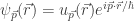
Fig. 2 Inside a crystal, the “free particle” electron states are described by a slowly-oscillating plane wave (blue curve) that is modulated by Bloch functions (black curve), which describe the electron’s attraction to the atoms (red and blue circles) within the repeating unit cell of the crystal. For a given momentum state, the electron probability density (shaded black areas on the left) is shared among the atoms within the unit cell in way that can depend on the momentum $\vec{p}$ . The Berry connection $\vec{X}$ is a vector that can be thought of as the centroid location of the electron within the unit cell, and it varies as a function of $\vec{p}$ .

Imagine now the hypothetical process of accelerating and then decelerating an electron in such a way that the electron returns to its initial momentum. During the course of this cyclic process the electron traces out a path $P$ in momentum space, and its final state is identical to its initial state except for a possible overall phase factor. This phase is an example of what is called a Berry phase and its value is

$\gamma_P = \frac{1}{\hbar} \int_P \vec{X}(\vec{p}) \cdot d\vec{p}$

(This expression for the phase is analogous to how a particle traversing a path in position space experiences a phase shift $\frac{1}{\hbar} \int_{P'} \vec{p} \cdot d\vec{x}$ , equal to the number of wavelengths in the path multiplied by $2 \pi.$ ) Traversing the path $P$ in the clockwise and counterclockwise directions leads to opposite signs for the phase $\gamma_P$ , since the direction of momentum change along the path is opposite in the two cases.

Fig. 3 The set of all possible momenta p for electrons within the crystal defines a Brillouin zone (denoted BZ, and illustrated for a 2D system by the black square). Opposite edges of the BZ describe the same wave function, and therefore are equivalent to each other. The Berry connection $\vec{X}$ is a vector field within the BZ (black arrows). If an electron is accelerated and decelerated along some closed path P (red loop), its wave function acquires an overall phase $\gamma_P$ whose sign depends on the direction of the path, clockwise or counterclockwise. A closed path along the BZ boundary gives an overall phase that must be a multiple of $2 \pi$ . This requirement can be seen as a consequence of the ambiguity in the direction of the path. For example, the thick red arrow at the top boundary is equivalent to the dashed blue arrow at the bottom boundary, and thus the path around the boundary can be described as either clockwise or counterclockwise.

The Berry phase becomes particularly instructive if we consider how it behaves for paths on a closed two-dimensional (2D) surface of momenta. For example, the Brillouin zone of a 2D system effectively acts like a closed surface because opposite edges of the zone are equivalent to each other. Consider, in particular, the path shown in Fig. 3, which traverses the Brillouin zone boundary of a 2D system. Traversing this path in the clockwise direction yields some Berry phase $\gamma_{BZ}$ , while the counterclockwise direction gives $-\gamma_{BZ}$ . However, because opposite edges of the zone boundary describe physically equivalent states, the clockwise and counterclockwise paths must produce equivalent changes to the wave function. The only way this requirement can be satisfied is if either $\gamma_{BZ} = 0$ , or $\gamma_{BZ}$ is an integer multiple of $2 \pi$ , so that the phase factor multiplying the wave function becomes equal to unity. This quantization of the Berry phase in units of $2 \pi$ can be turned into a more exact analog of the Gauss-Bonnet theorem by using Stokes’ Theorem to relate the contour integral along the boundary of the Brillouin zone to a surface integral across the entire Brillouin zone. This procedure gives

$\frac{1}{2 \pi \hbar^2} \int_{BZ} \Omega \ d^2p = C$

where $\Omega = \vec{\nabla} \times \vec{X}$ is called the Berry curvature, and $C$ is an integer called the Chern number.

One can notice that, even though local symmetries do not define the Chern number, having $C \neq 0$ requires that certain symmetries must be broken. In particular, one can see from Fig. 3 that within the Brillouin zone of a system with nonzero Chern number the momenta $+\vec{p}$ and $-\vec{p}$ are not equivalent, in the sense that they have different values of the Berry connection $\vec{X}$ . Such an inequivalence requires the system to break the symmetry with respect to inversion (inverting the spatial coordinates of the system) or time reversal (playing electron trajectories backward in time). Thus, the search for topological materials has largely focused on materials that break one of these two symmetries. In fact, as we show below, only systems with broken time reversal symmetry can have a nonzero Chern number, and breaking inversion symmetry alone is insufficient. However, the coupling between electron spin and momentum may allow a given spin species (up or down) to have a nonzero Chern number, so long as the two spin-resolved Chern numbers sum to zero.

Below we discuss this idea and other implications of electron topology, as well as its generalization to 3D systems.

Implications of Topology

One can notice from Fig. 3 that a nonzero Chern number implies a “winding” or “self-rotation” in the structure of the electron wave function. This self-rotation is associated with a physical angular momentum for electrons. For example, if one imagines making a wave packet using states from some particular region of momentum space, one sees that there is a relation between the position (within the unit cell) and the momentum of the states that comprise the wave packet. This relation between position and momentum implies an angular momentum for the wave packet that depends on the local Berry curvature. In this sense the Berry curvature is again like a magnetic field, created by a broken symmetry in the material itself rather than by any external source, in that it gives electrons an angular momentum.

The analogy of Berry curvature to magnetic field can be made more precise by considering the effects of an applied electric field $\vec{E}$ , which accelerates the electron momentum at a rate $\dot{\vec{p}} = -e \vec{E}$ , where $-e$ is the electron charge. If the local Berry connection $\vec{X}$ has a finite curl, then, as the electron accelerates, its centroid location shifts in the transverse direction. This shifting of the electron in the transverse direction is called the anomalous velocity, and is given by

$\vec{v}_A = - \frac{1}{\hbar} \dot{\vec{p}} \times \vec{\Omega} = \frac{e}{\hbar} \vec{E} \times \vec{\Omega}$ .

In this way, the anomalous velocity is like the E-cross-B drift experienced by an electron in crossed electric and magnetic fields. Applying an electric field in a particular direction causes an electron to drift in a direction that is, in part, transverse to both the field and the direction of the (momentum-dependent) Berry curvature, which acts like a magnetic field.

One of the most striking implications of the magnetic field analogy arises from the motion of electrons at the boundary of a sample. In a conductor with no intrinsic Berry phase that is subjected to a magnetic field, electrons near the boundary perform “skipping orbits”, essentially rolling along the boundary in a direction that is defined by the magnetic field direction. No matter how the boundary is shaped, these skipping orbits persist, providing a single conducting channel for current to flow through. In a similar way, the self-rotation implied by a finite Chern number guarantees the existence of traveling edge states. In 2D electron systems with a magnetic field (and sufficiently high electron mobility), the skipping orbit states give rise to the celebrated Quantum Hall Effect, including a quantized electrical conductance whose value is completely universal. 2D materials with finite Chern number have this same universal conductance, even though no magnetic field is present.

In fact, the existence of a topological invariant for electron systems subjected to a magnetic field was first identified by Thouless, Kohomoto, Nightingale and den Nijs (TKNN) [4]. This topological invariant allows for a remarkable universality of the quantum Hall effect among different samples and materials. In fact, the TKNN invariant allows the universal constant $e^2/\hbar$ to be measured to more than 12 significant figures of accuracy, and it now forms the basis for the metrological standard of the kilogram [5]. The Chern number defined above can be thought of as a generalization of the TKNN result, such that any given material has a particular integer Chern number defined in the absence of any applied fields. Most of the materials we know of have $C=0$ , and the possibility of 2D materials with nonzero Chern number was one of the seminal insights of the topological age.

There is an important way, however, in which the edge states of a topological material can be different from the edge states of a quantum Hall system. In a quantum Hall system, the magnetic field breaks the time-reversal symmetry of the system, since the magnetic field forces electrons to turn in spiral trajectories with a particular handedness, clockwise or counterclockwise, that is set by the magnetic field direction. These spiral trajectories break time reversal symmetry since playing them backwards in time (without reversing the sign of the external magnetic field) produces motion that is inconsistent with the Lorentz force law.

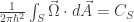
But it is possible to have a topological electron band, and its associated edge states, even in a material that has time-reversal symmetry. The key idea is to combine broken inversion symmetry in the material with a strong coupling between the electron’s momentum and its spin. For example, in the simplest case of a quantum spin Hall insulator, these two ingredients combine to allow the two different electron spin states to have nonzero but opposite Chern number. To see how this possibility can arise, consider that the time reversal operation also reverses an electron’s spin, so that, under time reversal, a left-going-spin-up electron becomes a right-going-spin-down electron. Thus, a topological electron band can retain time-reversal symmetry if the bands for spin-up and spin-down electrons have opposite Chern number (Fig. 4). Opposite Chern number means that the two spin species have opposite-moving edge states. This locking of the direction of the edge state to the spin is called the quantum spin Hall effect, and it was discovered experimentally in 2007 following its experimental prediction in 2003.

Fig. 4. A quantum spin Hall system has equal and opposite Chern number for its two spin species. (a) The Berry connection $\vec{X}$ winds in the opposite direction for up and down spins, giving $C = \pm 1$ , respectively. The system remains symmetric under time reversal, which simultaneously changes $\vec{p}$ to $-\vec{p}$ and ↑ to ↓ . (b) Edge states at the boundary of the sample move one spin clockwise and the other counterclockwise around the sample.

Ultimately, the locking of spin to momentum at edge states arises from the microscopic spin-orbit, or “ $\vec{L} \cdot \vec{S}$ ”, coupling that is present in atomic orbitals. Spin-orbit coupling arises when a fast-moving electron experiences a magnetic field in its reference frame due to the electrostatic potential of the nucleus, and the strength of this field varies as the fourth power of the atomic number. In topological materials with time reversal symmetry, strong spin orbit coupling combines with broken inversion symmetry to produce a Berry curvature and a finite Chern number for each spin, even in the absence of a magnetic field.

Topological bands in three dimensions

So far we have only discussed one example of a topological invariant: the Chern number in a 2D band, which gives rise to edge states very much like those in the quantum Hall effect. But a range of 3D materials have been identified with electrical properties that are protected by a topological invariant. These include the 3D topological insulators, which are largely made from narrow band-gap semiconductors with strong spin-orbit coupling [6]. In these materials, an electrically insulating interior coexists with surface states that form 2D metals on every free surface and have a similar locking of the electron’s spin perpendicular to its momentum.

The 2D Chern number discussed above can also be applied to understand another class of 3D materials: the Weyl semimetals. These materials have special points in momentum space where their “topological charge” is concentrated. To see why this happens, imagine defining an arbitrary closed surface S of momentum states within the 3D Brillouin zone of some material (Fig. 5). One can apply to this surface the same arguments about Berry phase that we used for the 2D case, and arrive at the conclusion that the Chern number associated with the surface must also be quantized. In particular,

$\frac{1}{2 \pi \hbar^2} \int_{S} \vec{\Omega} \cdot d\vec{A} = C_S$

where, $C_S$ is an integer that depends on the chosen surface $S$ and the integral defines a “flux of Berry curvature” through the surface. Since $C_S$ is an integer and cannot change continuously, slight distortions of the surface S cannot produce small changes to the integral. The only way for $C_S$ to change is by a discontinuous jump when $S$ is expanded to include a particular, special point in momentum space. Such points are monopoles of Berry flux, by analogy to the description of electric charges via Gauss’s law, and they always come in pairs of opposite charge. Materials that possess such monopoles are called Weyl semimetals, and the special points in momentum space are Weyl points.

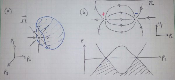
Fig. 5. A Weyl semimetal has monopole sources of Berry curvature and points where two different electron bands meet. (a) The Berry curvature $\vec{\Omega}$ is drawn as a vector field emanating from a special point in momentum space, a Weyl point. A closed surface that does not contain any Weyl points has Chern number $C = 0$ . If the surface is expanded to contain the point, it abruptly attains $C = 1$ . (b) Weyl points come in pairs with opposite charge, located at different momenta (above). At the Weyl point, two electron bands meet in energy (below).

From a materials perspective, Weyl points arise when strong spin-orbit coupling causes two bands of states with different angular momentum to coincide in energy. Since the orbital character of the wave function must change abruptly upon crossing from one band to another, Weyl points correspond to the locations in momentum space where the two bands touch. In the usual metals and semiconductors that comprise the majority of our electronic technologies, such touching of bands is unusual. Typically, electronic bands cannot coincide in energy because of the phenomenon of avoided crossing — the quantum phenomenon of hybridization of degenerate quantum states into symmetric and antisymmetric combinations that have different energies. However, it was recognized as early as 1937, in a paper by Conyers Herring that presaged much of modern topological band theory [7], that two electron bands could meet in energy because of “accidental degeneracies” that prevent the two bands from hybridizing. In these cases, a perturbation that removes an accidental degeneracy can destroy the band crossing point and open a gap. In Weyl semimetals, however, the Weyl points are protected by the quantization of the Chern number. Only a sufficiently strong perturbation, which effectively brings two oppositely-charged Weyl points together, can destroy the degeneracy and open a gap between two electron bands. Thus, a Weyl semimetal is a topologically-protected gapless system (a semimetal). Like the other topological materials, Weyl semimetals have intriguing surface states. In particular, the surfaces of Weyl semimetals exhibit Fermi arcs, or momentum states ranging from one Weyl point momentum to another [9].

Experimentally, the study of topological materials is progressing rapidly, with new compounds, even whole classes of topological materials, being discovered routinely. The initial discovery of 3D topological insulating behavior was made using angle-resolved photoemission spectroscopy (ARPES) in Bi_1-xSb_x, a mixture of two non-topological semimetals, each with spin orbit coupled bands, that produces a bulk semiconductor for 0.07 < x < 0.22 [12]. Since that discovery, many other topological insulators, as well as Weyl and nodal-line semimetals, have been identified. While ARPES remains a primary tool for revealing electronic band structures, the transport properties of topological materials are also being intensely studied, and raise the possibility of new device functionalities.

What technologies will topological materials enable?

The usefulness of many materials comes from their ability to either pass a current of some kind, or to prevent a current from flowing. For example, copper is useful because it allows electric current to flow freely down the length of a wire, while the polymer encasing the wire is useful because it blocks the current from leaking out. Other examples include materials for passing or blocking heat currents (like heat sinks on computer processors, or the insulating foam on the space shuttle) or filtering light (like the lenses on protective sunglasses, which pass some light frequencies while blocking others). Seen from this perspective, the “silicon age” arose because silicon can act as a kind of switchable valve, an “on/off switch” for electrical current. We know now that pure silicon is a good insulator, but if a “gate” voltage is applied to its surface it becomes an electrical conductor.

Thus, for developing new electronic materials, the main goals are usually filtering and sensitivity. The material should be able to selectively pass or block a generalized current (like silicon can selectively pass electrical current), or exhibit a strong response to some input (like silicon p-n junctions can turn light into electricity). In these questions of filtering and sensitivity, topological materials offer the promise of truly new technologies.

Topological materials can perform interesting kinds of filtering because of their Berry curvature. Since Berry curvature is a kind of winding or handedness that breaks the symmetry between clockwise and counterclockwise motion, topological materials can act like a doorknob, which “opens” when turned in the correct direction and blocks motion in the wrong direction. One striking application is in spin filtering. As illustrated in Fig. 4, the edge states in a topological insulator carry electrons with opposite spin in opposite directions. Such filtering is an essential ingredient for so-called spintronics, which aims to build electronic and computer technology based on currents of spin rather than charge [13]. The Berry curvature also implies that different directions of light polarization (clockwise or counterclockwise) couple differently to the electron material, and this effect can be used to create optical filters or logic circuits [14].

Topological materials are also unusually responsive to many kinds of applied fields, owing to their gapless, topologically protected electron bands. For example, the topological edge states associated with finite Chern number offer the promise of dissipationless current-carrying channels, a potential alternative to superconductors for some applications, perhaps even at room temperature. More generally, the topological protection of low-energy states in a topological electron band can be exploited in a number of ways, providing an advantage over conventional materials where the low energy states are often heavily distorted by disorder.

This topological protection of the electron band structure may be the reason why some topological materials exhibit enormous electrical mobility (i.e., a very large contribution to the current from each mobile electron) [15]. The Weyl semimetals can also have an extreme sensitivity to light, which may yield a new generation of photo-detectors and night-vision goggles [16]. Topological semimetals also promise an unprecedented thermoelectric effect, which is the ability to convert waste heat into useful electric power [17]. Finally, topological electrons have an unusually sensitive response to magnetic fields, including a wide spacing between quantum levels of the electron’s magnetic field orbit (Landau levels), and a strong reduction of electrical resistance when a magnetic field is applied along the current direction (the chiral anomaly) [18].

Whether these effects, or the myriad others that are currently being studied, will revolutionize our current electronic technologies remains to be seen. But what is clear is that ideas from topology have established themselves in materials physics, they have led us to predict and observe new materials and new phenomena, and they are here to stay. Who can tell how we will choose to name our current era in the decades to come?

References

[1] M. Riordan, and L. Hoddeson, Crystal Fire (W. W. Norton & Co., New York, 1997).

[2] L. D. Landau, Zh. Eksp. Teor. Fiz. 7, 19 (1937).

[3] F. Bloch, Zeitschrift Fur Physik 52, 555 (1929).

[4] D. J. Thouless, M. Kohmoto, M. P. Nightingale, and M. Dennijs, Physical Review Letters 49, 405 (1982).

[5] K. von Klitzing, Physical Review Letters 122,200001,(2019).

[6] C. Kane, and J. Moore, Physics World 24, 32 (2011).

[7] C. Herring, Physical Review 52, 0365 (1937).

[9] X. G. Wan, A. M. Turner, A. Vishwanath, and S. Y. Savrasov, Physical Review B 83,205101,(2011).

[10] C. Fang, H. M. Weng, X. Dai, and Z. Fang, Chinese Physics B 25,117106,(2016).

[11] F. Schindler, A. M. Cook, M. G. Vergniory, Z. J. Wang, S. S. P. Parkin, B. A. Bernevig, and T. Neupert, Science Advances 4,eaat0346,(2018).

[12] D. Hsieh, D. Qian, L. Wray, Y. Xia, Y. S. Hor, R. J. Cava, and M. Z. Hasan, Nature 452, 970 (2008).

[13] I. Zutic, J. Fabian, and S. Das Sarma, Reviews of Modern Physics 76, 323 (2004).

[14] K. F. Mak, D. Xiao, and J. Shan, Nature Photonics 12, 451 (2018).

[15] T. Liang, Q. Gibson, M. N. Ali, M. H. Liu, R. J. Cava, and N. P. Ong, Nature Materials 14, 280 (2015).

[16] C. K. Chan, N. H. Lindner, G. Refael, and P. A. Lee, Physical Review B 95,041104,(2017).

[17] B. Skinner, and L. Fu, Science Advances 4,eaat2621,(2018).

[18] A. A. Burkov, Journal of Physics-Condensed Matter 27,113201,(2015).

[19] B. Bradlyn, L. Elcore, J. Cano, M. G. Vergniory, Z. Wang, C. Felser, M. I. Atoyo, and B. B. A. Bernevig, Nature, 547, 298 (2017).

The Physics Olympiad, and finding community

July 16, 2019

by Brian

When I was in high school I spent about 2 hours after school every day running track. This was, on the face of it, an unpleasant thing to do. Running is literally painful, and I devoted something like 10% of my waking life to it.

So why did I do so much running? It turns out that there were more or less three reasons. First, I was an ambitious kid, and competitive running provided an outlet for that ambition. Second, I got to experience the joy of acquiring a new skill, and seeing myself improve at something that had previously been difficult. Third, and perhaps most importantly, joining the track team gave me access to a social community. I made friends (including across the normal lines of class and race that tend to divide students), I had adventures, and I matured as a social being.

These are all normal and healthy reasons for doing something that might otherwise seem unpleasant.

I bring this up because last month I spent two weeks at the training camp for the US team of the International Physics Olympiad. The twenty kids at this camp are among the smartest high school physics students in the country, and to arrive at this level they had to devote about 2 hours every day after school to studying physics.

This is, on the face of it, an unpleasant thing to do.

I think that their reasons for studying physics so intensely are similar to my reasons for running track. These are mostly ambitious kids, who enjoy doing something competitive and acquiring a new skill. But what a surprise and a joy it has been for me to discover that physics can also bring high school kids community. These kids (seem to have) made deep and lasting friendships at camp, and I am learning that there is a whole world of physics clubs and camps and internet forums that I was previously blind to. Physics seems to be central to their social life in a way that sports was to me, and is to so many other kids.

And the truth is that studying physics has rewards that are probably more real and long-lasting than the ones that come from sports. Even if these kids don’t become physicists by profession, they will have had the experience of learning difficult but exciting things and solving difficult but exciting problems. And that’s the sort of thing that shapes your opinion about the world and about yourself in a very positive way.

It’s hard for me to discuss the physics olympiad without gushing about the staggering intelligence and technical competence of these kids. They are literally, without exception, 4-5 years ahead of where I was when I graduated from high school. I saw them quickly solve physics problems that I would have struggled with as a grad student, and which even today took me a while to figure out. While preparing the first practice exam in camp, I wrote a problem that I thought was clever and tricky, using some logic I had learned in grad school. And then when I graded the practice exam I found that their median score on the problem was 19/20.

You know, I grew up to be a physics professor. So I can’t even predict what their opportunities will be.

If anything, I worry that these kids are so clever that they will have a hard time emotionally when they first encounter an interesting physics problem that can’t be solved at all. They have become so used to being able to solve tricky and clever problems, that perhaps when they get their first taste of physics research — of encountering a problem that might not even be well-posed, and might not have a solution — it will be difficult for them emotionally. Or, even worse to imagine, they could take it as a sign that they’re not really smart enough to do physics, when in fact the issue is with the problem and not the problem-solver.

A friend of mine (a physics professor, whom I’ll call Val) once told me the story of some of his high school classmates. Val had gone to some kind of magnet school in Croatia, and he had several brilliant classmates. These classmates always seemed to solve physics problems effortlessly, while Val himself struggled continuously. He felt, in the end, that he got through high school physics only by leaning on his friendships like a crutch. Eventually they all went to college together, and the brilliant friends remained brilliant and breezed through everything, while Val continued to struggle with each concept and always felt like he was just barely eking by.

After college they all went to grad school in physics, and suddenly the problems they were working on got truly hard. These problems required months, semesters, or even years of slow and painful thinking, trying many wrong approaches before eventually stumbling on something that worked (or, perhaps, eventually giving up and trying something else instead). For Val, this was natural — this was how physics had always been for him. But for the brilliant friends this kind of frustration and lack of progress was oppressive. They got discouraged, and eventually lost enthusiasm and left physics altogether.

All this is to say, I hope that physics isn’t too easy for these kids. I hope that they love it even when it feels unclear, frustrating, and slow. This way, when it really those qualities in earnest, they can still love it.

Of course, if they leave physics to do something else, that’s fine too.

Crowding around the blackboard to learn some thermodynamics from head coach JJ Dong

Powering through one of the many practice exams

I probably need to address the elephant in the room here: demographics. Of the 20 students who qualified for the physics olympiad camp (on the bases of two rounds of exams), 16 were Chinese-American, 3 were Indian-American, and one was Caucasian. There were 19 boys and 1 girl.

But racial and gender biases weren’t the only demographic trends on display. There was also an overwhelming representation of private schools and magnet schools, even though the vast majority of high schoolers in the USA attend non-specialized public schools. Certain “powerhouse” schools, in particular, seem to have multiple students qualify for camp every year.

As far as I can tell, these biases in representation come down to who is being encouraged to study physics, and who is being invited into the corresponding communities of physics. When I was in high school, for example, I had no idea that competitive physics was a thing, much less that there was a world of clubs, camps, and internet forums devoted to it. Maybe if I had known I would have chosen my hobbies differently.

At the moment this information seems to pass through certain communities of parents by word of mouth, and then the parents in turn motivate their children. Part of the problem, then, is on us, the coaches and organizers of the physics olympiad. We need to do a better job of getting the word out, and making people aware of the fact that there is a whole world of recreational physics (and recreational math and science, more broadly) available to kids. It can be as rewarding and engaging as any other hobby, and any other community.

But part of the problem is more intractable then a simple increase in advertising. If, as a teenager, you want to become a great runner, you probably need access to a good team and a good coach. So it is with physics, too: you will be hard-pressed to become a great practitioner of competitive physics unless there is a community in your school that is ready to give you training, friendship, and opportunity.

So perhaps this blog post can serve as an exhortation both to students and to teachers/administrators. Be aware that there is a whole world of recreational/competitive physics out there, and this is a world that is challenging, exciting, and comes with long-lasting benefits. Think about finding a way to engage with this world, or helping to open a path that enables others to do so.

For more information about the USA Physics Olympiad program, read this page: https://www.aapt.org/physicsteam/2019/program.cfm

You can read about the 2019 USA Physics Olympiad team here: https://www.aapt.org/physicsteam/2019/team.cfm

The 2019 Physics Olympiad (in Tel Aviv, Israel) is currently wrapping up. The results should be announced very shortly. But for the moment I can say that all five members of the traveling team performed brilliantly!

UPDATE: The results are released: https://www.ipho2019.org.il/results/

Congratulations to gold medalists Vincent Bian and Sean Chen, and to silver medalists Edward Lu, Albert Qin, Sanjay Raman!

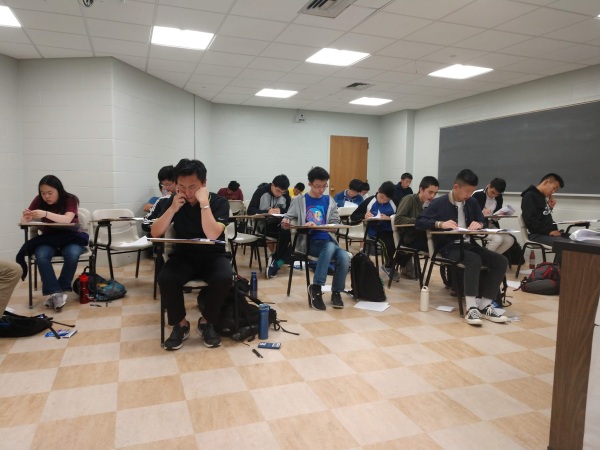
Physics goes to Washington

The camp ended with everyone treating their physics textbooks like yearbooks

What it means, and doesn’t mean, to get a job in physics

March 25, 2019

by Brian

I have some reasonably momentous personal news: I got a job.

And I don’t just mean that I got a job, in the same sense that I’ve been employed doing research ever since getting my PhD. I got the job: the ostensibly permanent faculty position that so many of us have aspired to (and agonized over) since undergrad.

I have accepted a faculty position in Physics at Ohio State University. I’ll begin in January.

It isn’t my intention to brag here. But I should probably make the point that this job is a big deal for me. OSU Physics is an extremely good department, with great students and something like ten faculty members whose work I admire and whom I am eager to learn from. When you’re angling for a faculty position, you can really only hope to end up with a couple of colleagues like this, so for me this job is an embarrassment of good fortune. It’s not an exaggeration to say that this is exactly the kind of job I’ve dreamed of having ever since I decided that I wanted to be a scientist. I am very excited.

But I should also make the point that getting this far was difficult, long, and not particularly likely. My goal in writing this post is mostly to give a postmortem dissection of my career trajectory, for the benefit of current students who are thinking of following a similar path. I want to try and point out, as honestly as I can, which things I did right, which things I did wrong, and the ways in which I got lucky that enabled me to finally have a secure career in academic science.

A caveat: there is a risk when writing this kind of reflection of building up the tenure-track faculty position as some kind of ideal. That is, there is a danger of making it sound like getting a faculty job is “making it” while other options are “failing to make it”. I don’t mean to do that. There are lots of exciting things to do with a physics degree besides going on to be a physics professor. And there are plenty of people who were smarter than me and/or better at physics than me who went a different direction. To name a few, some friends and colleagues of mine went on to be: research scientists and engineers, data scientists, software engineers, financial analysts, technical writers, science journalists, teachers, and intelligence analysts. Many (perhaps even most) of these careers might be more rewarding or more challenging than the standard tenure-track professor job. But I can only comment on the path I followed myself.

Beware: this is probably the longest post I have ever written.

What are the odds?

I remember, as an undergrad, deciding more or less immediately that I wanted to try and be a physics professor. It was an exciting thought, but the one that immediately followed it was: “what are the odds?” I remember looking through the faculty roster at my university and seeing everyone’s listed undergraduate and graduate alma mater. It was pretty much a parade of Harvard, Princeton, MIT, Caltech, Stanford, Berkeley, MIT, etc. “Well,” I thought, “I’m at Virginia Tech. So what does that mean about my chances?”

From that moment on I pretty much operated under the assumption that I wouldn’t achieve my goal. But I decided that it was worth trying anyway, because I would at least get to have a physics-themed adventure along the way. And once you get a PhD in physics people seem to generally believe that you’re a smart person, and are willing to hire you for a range of different technical jobs (which is true; see the list of alternate jobs above). So my plan was to go to grad school in physics and then reassess from there, with the expectation that I would probably end up in some kind of non-academic, technology-oriented job.

The basic timeline of my academic path is like this:

I started college at Virginia Tech in the fall of 2002, and graduated in the spring of 2007 with degrees in physics and mechanical engineering. (In high school I had thought I wanted to do robotics, and in college I was too stubborn to drop the mechanical engineering degree that I initially declared.)
I started grad school at the University of Minnesota in the summer of 2007, and completed my PhD in the summer of 2011. (This is an unusually short duration; see comments below.)
I stayed in Minnesota for two years as a postdoc, then went to Argonne National Laboratory in 2013 for a second postdoc. I spent two years there, which included applying for a number of faculty jobs that I didn’t get.
I started a third postdoc at MIT in 2015. I applied extensively for faculty jobs during my time at MIT, but I wasn’t able to find a position before my appointment ran out in 2018. I was fortunate enough to find someone else willing to pay for me for an additional year, and in March of 2019 I landed the job at Ohio State.

So the chronological recap is:

5 years of undergrad
4 years of grad school
8 years of postdoc (at three different locations)

It’s a long road, friends.

I would say that, in my field, 8 years as a postdoc is longer than average. And, in fact, I was more or less considering that this year was my last chance. In an email, my PhD advisor had warned me that “your career will not survive another postdoc”, and he was probably right.

But 8 years is also not some extreme outlier. The average time spent as a postdoc (again, in my field) might be something like two postdocs and 5 or 6 years. Three postdocs is usually considered an upper limit, and people who don’t have a permanent job by the end of their third postdoc are often passed over or viewed with suspicion.

Along the way I had to make many, many job applications. Here’s the total count, along with the year of applying (in parentheses):

10 grad school applications (2007)
1 (2011) + 12 (2013) + 8 (2015) = 21 postdoc applications
1 (2012) + 16 (2015) + 7 (2017) + 33 (2018) + 42 (2019) = 99 faculty applications
1 (2012) + 3 (2015) + 6 (2018) + 5 (2019) = 15 faculty interviews

I probably don’t need to say that applications are exhausting and dispiriting. Faculty applications, in particular, are very time-consuming, and an actual faculty interview is brutal. My general rule of thumb is that during any year in which you are applying for a new (academic) job, you will lose about a third of your total productivity to the process of applying and the stress of worrying about how the application will turn out. Add together the years above and the implication is that I lost something like two solid years of my life to applications.

With each year of failure on the faculty job market, I got a little more anxious and a little more desperate. During the last two years, I often had to specifically justify why so much time had passed since my PhD. For example, during a Skype interview this year I was asked directly by the committee “It’s been a long time since your PhD; why don’t you have a job yet?” (they did not invite me for an in-person interview). More than once someone called my PhD advisor to ask for a justification as to why so much time had passed since my PhD.

In the end, I got a great job at a great institution. But I had to endure nearly 100 rejections and ten failed interviews first. There were many moments along the way when I thought I was looking at the end of the line.

I once heard it said (by a tenured professor) that there’s no point in stressing about jobs, because in the end all the “good people” get faculty positions and everyone else winds up with a lucrative tech-related career. This kind of dismissive and self-serving narrative seems completely inconsistent with my own observation. Luck seems to play as big a role as anything else.

In the remainder of this post I want to spell out the many ways in which I was the beneficiary of luck and kindness from others. But let me first try to be at least a bit positive and constructive, and outline the things I think I did correctly.

What I did right

I prioritized conceptual understanding over technical skill

When you’re a young student or postdoc, your first years are usually marked by a long struggle to gain some technical skill or competency. As soon as you attain this skill at the level required to produce publishable research, it’s very tempting to just rush to apply the skill to all the problems you can find. This kind of approach maximizes your instantaneous productivity at a time when you feel desperate to be as productive as possible.

But ultimately this is a dangerous approach. Because in order to get a job, you need to impress people in person, and not just on paper. And what impresses people in person is the ability to understand what they are working on, to ask intelligent questions, and to teach them some idea that they didn’t previous understand. If you can’t do this, and you instead come across as a “narrow professional” in an interview or a discussion, then people can be dismissive of you as a scientist.

In this sense I did the right thing by prioritizing a broad, conceptual understanding of physics over a narrow and virtuosic expertise. In my case this was sort of an accident; I did the former because I had a short attention span and easily got bored by doing the same thing repeatedly. It turned out, in the end, to be a good career move.

I learned how to talk about physics, in addition to learning how to do physics

The great theorist Anatoly Larkin used to say that there are two kinds of physics: written physics and oral physics. What I think he meant is that there are two distinct skills you need to acquire as a scientist: (1) the ability to do calculations or experiments, and (2) the ability to talk conceptually about science with your peers. As a student you often feel like the second skill will come naturally once you acquire the first. That is, you think that once you can produce science you will naturally be able to talk about it clearly with others.

But this isn’t true. Getting good at talking about science requires a concerted effort. You have to work and practice to be able to describe things to others in their simplest terms, or be able to make analogies and construct clear examples, or be able to approach an idea from multiple perspectives in case the first perspective doesn’t take. Without these skills your scientific career will almost certainly fall apart sooner or later, because “oral science” is the only way to impress people and forge collaborations.

Luckily for me, this skill was something I prioritized, mostly because I thought talking about physics was so much more fun than doing calculations. In fact, I created this blog (almost exactly ten years ago, during my second year of grad school) mostly as an outlet for my desire to “talk about physics” as distinct from “doing physics”. I’m very glad that I did.

I worked hard to make good talks

A common piece of advice given to grad students and postdocs is “until you get a permanent job, treat every talk like a job talk.” I’m not sure that this is a helpful thing to say, since it’s inclined to make you feel nervous and pressured at a moment when you need to feel relaxed. But it is true that anytime you give a talk you are building your reputation a little bit, and you are building up skill for a future job application. So take your talks seriously.

For me personally, a good talk is one that I learn something from. So when I’m designing a talk I always try to have at least one moment where I explain/derive some result in a clever or striking way. This “clever result” doesn’t have to be something that came out of my own research; it can be someone else’s idea, old or recent (and you should, of course, generously credit the person who originally came up with it). But the best way to make a scientist like you is to teach them something in a clear and clever way. Don’t pass up that opportunity lightly.

The best talks also have a narrative flow to them. In particular, they clearly set up a dilemma before resolving it. Before you tell the audience whatever new result you have, you need to make them feel uncomfortable about not knowing it. Don’t let your talks be just a summary of what you did.

I made friends in physics, and I put a lot of effort into maintaining those friendships

This may seem a little cynical, but it’s absolutely true: your friendships in science matter enormously to your career success. The people in your field who like you are the people who will provide you with opportunities – invitations to give lectures, invitations to conferences, opportunities to collaborate, positive reviews on your papers, etc. Having friends also just makes the process of doing science more fun.

I am not naturally a socially skilled person, so my method of making friends usually exploited the one interest I knew we all had in common: physics. Many of my friendships started by striking up a conversation about physics. Teaching someone an idea in a clear way is a great way to make a friend, but so is asking them to teach you.

I approached well-known, established people for mentorship and collaboration, and I tried to do good work for those people

This one mostly comes down to courage. Any field has its famous people, who are known for some body of great work. It’s easy to feel intimidated by these people, or to feel like you shouldn’t bother them. But if an opportunity comes to discuss science with such a person, or to collaborate scientifically, you almost have to take it. Eventually, to get a real job, you need to have (multiple) well-known people write you good letters of recommendation. The only way to get there is to boldly take the opportunities to work with those people whenever you get the chance.

Just remember, of course, to have the requisite humility. Be confident about the things you know how to do, and you should even be willing to “teach” some great person where you are able. But don’t ever pretend to understand something you don’t. Don’t pontificate and don’t pose. Most great scientists are happy to explain things, even if they seem embarrassingly basic to you. But they probably won’t tolerate posers.

When I found people who were smarter than me, I tried to learn from them

As an early-career scientist, you will continually find yourself running into people who are both younger and smarter than you. Given the omnipresent job anxiety, it’s easy to let these people make you feel deflated, anxious, or even resentful. Resist those urges as much as possible, and instead try to get these people to teach you things that you don’t know. This kind of earnest friendliness is a wonderful thing for them and for you. Some of my best friendships in science have been made this way.

I was generous, open, and friendly, and avoided being competitive or proprietary

This one can feel surprisingly hard, because there are so many great people competing for a very limited number of permanent jobs. So you can easily feel pressure to be overtly competitive with your peers – anxiously guarding your work away from them, competing for the attention of famous professors, or even “stealing” problems from others. But this kind of behavior will put you on people’s bad sides very quickly. On the other hand, being generous with your time and labor, open with your results, and friendly toward everyone will help you make much-needed friends.

I made an effort to be creative

In some fields, and in condensed matter physics in particular, there are topics that suddenly get “hot”, and a huge fraction of people suddenly start working on the trendy new topic. This leads to a deluge of work that is done quickly and obviously: people want to be first to establish some new result or stake some claim before others do. And the truth is that you probably need to spend some time doing this kind of work (see another comment below). But I personally tried to set aside at least some time to do creative work that wasn’t directly aligned with any trend or established field. This work wasn’t always cited very well, but I think that in the end people respected me for it. And it allowed others to see that I was someone who was willing to think creatively and across fields. While such broad-mindedness is often a secondary consideration in hiring decisions, it is a purely positive one, and it’s the sort of thing that people like to have in a colleague.

I was willing to sacrifice from my personal life and my personal relationships when necessary

This point is the saddest one to discuss, but I am trying to be as blunt and honest as possible.

I have been married for ten years. But I have lived apart from my wife for three of those years. If I hadn’t been willing to sacrifice from my marriage in this way – if I had insisted that I can only take jobs in cities where my wife is also employed – then I would almost certainly not still have a viable academic career.

This state of affairs is unfortunately very typical in academic science, unless one of two people in the relationship make a decision to abandon much of their career ambition and follow their spouse.

What I did wrong

I finished my PhD quickly

This one feels counterintuitive, but it’s an important point.

The first few years of my PhD were atypically productive, thanks to an unusually fortuitous match with my PhD advisor (more on this below). Three and a half years or so after entering grad school, I had authored or coauthored something like 12 published papers. So my advisor and I both decided that I had enough work to defend a PhD thesis, and I graduated after my fourth year. I was angling to stay in Minnesota longer while my wife finished her degree, so I transitioned smoothly to a postdoc with the same group.

Graduating “early” like this seems like a uniformly good thing to do. But it isn’t. The reason is that when you apply for future jobs people will judge your productivity on a sliding scale, with increasingly high standards based on how many years have passed since your PhD. On the other hand, no one really pays attention to how long the PhD lasted. So, all other things equal, a candidate who publishes 16 papers in their PhD looks significantly more impressive than a candidate who publishes 12 papers in their PhD and another 4 in their first postdoc, even if the two candidates started grad school at the same time.

So my advice is this: if you find yourself being very productive in the later years of your PhD, and if your goal is to get a faculty position, then draw those years out as long as you reasonably can. Be productive, write papers, learn a lot of things, give talks, etc., as a grad student. Because when people judge you, you want them to be able to think “wow, that person is such a great scientist, and they’re still just a grad student!”

I avoided fashionable topics

I know, I know, this one sounds like the most self-serving excuse for not having highly-recognized work. (My publication record at the time of being hired is decent, but probably below the level that is typical for a faculty hire at an Ohio State-level university.) There is a very common (and annoying) complaint among scientists: “I did responsible and deep work, but I never got the recognition I deserved because it wasn’t trendy at the time.”

In my case, though, I can’t claim that I avoided trendy topics because I was doing “deeper” work, necessarily. There were other reasons for my reluctance to jump into fashionable and fast-moving fields. And if I’m being honest, these reasons are not particularly flattering.

One reason for my reluctance was a kind of intellectual anxiety, or a lack of confidence. When a field is just emerging, everything feels new and confusing, and it can be very intimidating to try and jump in. You feel overwhelmed by how much you don’t know, and rather than buckle down and try to learn it all, it’s easy to just stay away and work on things you already know. But this is a missed opportunity. A field that is developing rapidly is also a field where people are learning rapidly, and if you stay away you will probably be learning less than you could be.

I think also that I abhorred the lack of clarity that predominates in a developing field. There is a sudden torrent of papers that make confused or contradictory claims; people rush to do experiments that aren’t properly controlled or properly understood; people rush to do calculations that are based on questionable assumptions. I hated wading through all that muck, and I allowed myself to justify staying away from it because I didn’t want to have to do the work of generating a clear perspective for myself.

This was also a missed opportunity, both to grow as a scientist and to establish myself as someone who is capable of creating clarity in a field where it was previously lacking.

I didn’t spend enough time reading new papers

There is a website called the arXiv, on which people post drafts of their new scientific papers, usually before submitting them to a journal for review. The arXiv is sort of the lifeblood of current events in physics. Most established physicists scan through the arXiv every night, catching up on the latest developments and looking for inspiration.

I tried to maintain an arXiv-reading ritual, but the truth is that I hated it. Looking through dozens or hundreds of papers every night, most of which seemed confusing, incomprehensible, and/or completely boring, was too hard for me emotionally. It made me feel overwhelmed, and I would start questioning why I was doing this and why I was in this profession at all. Eventually I just gave up, and I never really developed any kind of routine for reading new papers as they came out. I fell back on merely going to talks and conferences, talking to people at lunch, and googling things as needed.

This reluctance to read papers cost me significantly. I was usually late to learn about new developments, and I missed many opportunities to collaborate with others or provide them with information or references (including to my own work) that would have been helpful.

I allowed my work to become scattered, rather than focusing on a single field

When it comes to science, I have a bit of a short attention span. A scientific field is always most exciting to me when I am just learning its central ideas, and once I understand those I am easily distracted by some other field.

This tendency isn’t bad, necessarily, since it leads to rapid learning and creative thought. But when you are a young scientist you need for some community to recognize your work, and to know you personally. In my early years I made the mistake of scattering my work across many disconnected scientific communities. Suddenly, I found myself four years past my PhD and I realized that there was probably no scientist alive who would have read more than 3-4 of my 25 papers. This was a problem, and it probably delayed my employment significantly.

I insisted too often that people explain things in my terms, rather than learning to understand things in their terms

I realized relatively quickly that I had a “style” of doing physics. I had a particular way of thinking about things, which was based on intuitive pictures and simple math. This is not a bad thing; I have come to realize that my style has real value, and many people appreciate it.

But a lot of the time I would insist on thinking only in this style. When someone was trying to explain some idea to me, I would insist on parsing it in this way, asking lots of questions and forcing them to rephrase what they were saying until I could understand it and derive it in my natural language.

While understanding things in your own terms is probably essential to learning, it’s also true that I should have put in the work of learning how to think in multiple different ways at once. There were a lot of popular, “formal” ways of thinking in theoretical physics that I was slow to develop, to my detriment.

I didn’t prioritize my career over my wife’s career

This point, again, is difficult to admit, and even embarrassing, both for myself and for my profession.

Starting with graduate school applications, my wife and I made career decisions jointly. We always tried to weigh the options and choose the one that maximized the combined net benefit to her and to myself. To me this is the obviously correct, human way to behave in any kind of partnership. But in some cases the human approach meant that I didn’t get my first option, and in an ultra-competitive field that always made me more than a little nervous.

I don’t want to overplay this point, because in the end I got a very good job, and it’s hard to imagine that I would have done significantly better in some alternate timeline. And I’m more than grateful for the sacrifices that my wife made for the benefit of my career, and for all the times when she didn’t get her first choice. But it’s also true that by the time I arrived at my postdoc at MIT, most of my peers were either single or had partners who had agreed to subordinate their own career ambitions to that of their physicist partner. It is usually true, with some rare exceptions, that if you want to be a professor you don’t get to choose where you will live, and that means that someone’s career will probably have to take priority.

Ways in which I was lucky

I was uniformly encouraged

I was something like 8 years old when I first thought it would be cool to be a scientist. From that point onward, I would occasionally tell people that this was my aspiration and I don’t remember anyone ever giving me a single discouraging word.

It wasn’t until adulthood that I realized what a big deal this is. When I told people that I wanted to be a scientist, and they were encouraging, it allowed me to believe in the reality of the future I wanted. When difficulties inevitably arose, I was able to view them as simply difficulties, rather than as evidence that I wasn’t intrinsically good enough.

I had undergraduate advisors who cared more about my future than about their own research

As a freshman in college, I picked a research advisor almost at random. I asked the guidance counselor which professors wanted undergrad researchers, and then I went to the first person on the list. That the first name on the list was Beate Schmittmann was maybe my first really lucky break in physics.

Dr. Schmittmann was unusual in that, in her interactions with undergrads, her only real motivation was to introduce them to research and give them opportunities. Amazingly (in retrospect), she never tried to use my (inconsistent) labor to advance her own research. She introduced me to physics ideas, took me to conferences, and helped me through applications without ever asking for publication-quality work from me.

And I had a number of other professors who treated me this way: Dr. Bruce Vogelaar (also at Virginia Tech) introduced me to experimental particle physics, and gave me a number of really wonderful opportunities even though I was ultimately terrible at both particle physics and performing experiments. I did summer internships at MIT and at CERN, and it is really humbling in retrospect that anyone devoted any kind of resources to someone as inept as I was.

I ended up with a PhD advisor who (1) was famous, (2) really cared about teaching me, and (3) worked relentlessly to find me opportunities

By far the biggest piece of luck I had was in who I had as a PhD advisor. When you’re an undergraduate applying to grad schools, you have no understanding whatsoever of what makes a good advisor, or who the people are at the schools you’re considering. For the most part, you just look through people’s websites and see if they have any words or pictures that you like.

When I arrived at the University of Minnesota in the summer of 2007 I didn’t really know anything about the people there. I ended up working with Boris Shklovskii almost randomly – I chose condensed matter theory, and he was the first person who reached out to me. I also liked the titles of some of his papers.

But it turns out that who you have as a PhD advisor is the single biggest determiner of your academic success. Ideally, you want someone who is well-known and well-connected, who will provide you with good topics to work on and opportunities to make yourself known, and who will take time to teach you. It is rare to get all three of these things, and I was extremely fortunate to have all of them.

Boris is a rare and singular person in many regards. He is such an uncommonly clear scientific thinker, and he devoted an enormous amount of his time to me personally. All I can say is that I am exceptionally fortunate and exceptionally grateful for my time as his student, and I will have to write a proper post about him as a scientist some other time.

It turns out, though, that even having an advisor with all these qualities is not enough to make your PhD successful. You also need your advisor’s style of thinking and working to be compatible with your own. And it happened that Boris had his own unique style, which was remarkably closely aligned with the way I wanted to think about physics. So my good luck in that regard is really remarkable.

I went to the Boulder Summer School and made lots of friends, many (most?) of whom remained in academia

The biggest month of my early career came in the summer of 2013, when I attended the Boulder School for condensed matter physics. This was a month-long summer school, during which PhD students and postdocs could attend special lectures while living together in a dorm at the University of Colorado.

It is hard to overstate how important that summer was for me. Not necessarily because of the lectures (from which I learned much but retained relatively little), but because I suddenly found myself surrounded by exceptional young scientists, most of whom are still in academia. To be in that environment was so exciting, that all I wanted to do was hang out and talk about physics with them all day. It was during that summer that I really learned the joy of making friends with someone by teaching each other physics. We also did adventurous things, too, like go hiking and camping, but the real joy was the physics itself. Many of my best friends were made that summer.

I don’t know whether every year at Boulder School is like that, or whether I was part of an exceptionally good group. But if you are a student or postdoc, and you have the opportunity to go to a summer school like this one, I can’t urge you strongly enough to go. Go, make friends, and talk about science all the time. It will pay dividends for a very long time.

I got a postdoc position with an independent travel budget, and I used it to my full advantage

My postdoc at Argonne National Laboratory started in the fall of 2013, and it came with an unusual perk: a $20,000-per-year discretionary budget. This is extremely rare for a postdoc, and is probably a vestigial remnant of an arrangement that was originally designed to provide an experimentalist with equipment.

But I took full advantage of that budget. I traveled to give seminars at places that wouldn’t otherwise have had a budget for it. And I treated myself to a whole range of conferences both foreign and domestic. It was a great way to introduce myself to the wider scientific world, to make friends and to make myself known. And I also got to add a disproportionate number of “invited seminars” to my CV.

Someone was kind to me and gave me a postdoc job when I was floundering

In the spring of 2015 I was in something of a panic. Despite my rampant (mis)use of government funds, I couldn’t find a job. And to make the matter even more difficult, my wife was going to medical residency, which is governed by a tyrannical and completely non-negotiable matching algorithm. Predicting the outcome of the match is a hard thing to do, but after some agonizing it seemed like she was likely to be sent either to San Francisco or to Boston.

I think this was the first time when I really thought that I was done for. The outcome just looked too bleak: I couldn’t bear to be apart from my wife any longer, and I couldn’t see any way to get an academic job in either of those cities.

One night I was despairing to a Boulder School friend of mine who was a grad student at MIT, and he said “why don’t you just ask my advisor for a job?” This had never occurred to me. My friend’s advisor was an intimidating Russian theorist who was widely regarded as a genius. I had, in fact, had a few good (but short) conversations with him, at a couple conferences and during a self-invited visit to MIT. But I never expected that he would deign to hire a (very) non-genius like me.

Nonetheless, I wrote to him one night and said [verbatim] “I find myself these days coping with a sort of tricky two-body problem, and recent developments are making me very motivated to find a job somewhere in Boston. … Do you know of anyone in Boston who is looking for a postdoc that might be interested in me?”

The very next day he said “I’ll make some inquiries and get back to you”, and within two weeks I had an offer letter for a postdoc at MIT.

I can hardly tell you what a miraculous event this was. My wife and I got to live together, and I got an office on the Infinite Corridor at MIT.

I should admit at this point that I had harbored an unrequited crush on MIT for a long time. Up to that moment, I had applied to be at MIT five times – for undergrad, for grad school, for a summer program, and for two postdoc positions – and had been rejected every time. In the end I got a position that required no application at all: just an email and a bit of nepotism.

I befriended people at MIT who became great scientists

The year I arrived at MIT there was an unusual cohort of brilliant and friendly young postdocs. I became fast friends with many of them, and have developed friendships that I truly cherish. I learned enormously from them, wrote papers with them, sang karaoke and went on hikes with them, and I can’t tell you how excited I am that I get to have a scientific career in parallel with them. Most of them have now gone on to faculty positions of their own.

Someone was kind to me and kept me on when I was about to fail out

I should say, finally, that even after making it to MIT it was not at all clear that I had “made it” into a permanent scientific career. During my second year at MIT I applied to seven faculty positions and didn’t get a single positive word in return; not an interview or a phone call. I tried again the next year, ostensibly the last of my three-year postdoc, and applied essentially everywhere that had even a remote chance of working for both me and my wife. The initial returns seemed good: I got six interviews at six good universities. But in the end I was not quite good enough anywhere, and after a protracted period of “maybe” from a few schools (and a few quicker rejections from others), I found myself completely without a job, seven years past my PhD, and with just a few months before my current job expired.

At this point I really thought the game was up. I was preparing my exit strategy, and trying to line up interviews in the private sector. But a different professor happened to hear about my predicament, and he offered to pay for me for one more year. This gave me one last chance at the academic job market, and the rest, I suppose, is history.

What to make of it all

If you are a young grad student or postdoc in science, reading this (overlong) account, I don’t know how you should feel. On the one hand, my career arc thus far has been a great adventure. If I saw someone else getting excited about the prospect of such an adventure, it would be easy for me to get excited with them.

But this arc has also been a difficult and very tenuous journey, generously supported by good fortune and by kindness from powerful people at just the right moments. If your decision upon reading this account is to avoid the whole mess altogether, then that seems as rational to me as anything else.

How thick is the atmosphere? A derivation of the Boltzmann distribution

July 14, 2018

by Brian

Let’s talk about a small question as a way of introducing a big question.

How thick is the atmosphere?

How far does Earth’s atmosphere extend into space? In other words, how high can you go in altitude before you start to have difficulty breathing, or your bag of chips explodes, or you need to wear extra sunscreen to protect your skin from UV damage?

You probably have a good guess for the answer to these questions: it’s something like a few miles of altitude. I personally notice that my skin burns pretty quickly above ~10,000 feet (about 2 miles or 3 km), and breathing is noticeably difficult above 14,000 feet even when I’m standing still.

Of course, technically the atmosphere extends way past 2-3 miles. There are rare air molecules from Earth extending deep into space, becoming ever more sparse as you move away from the planet. But there’s clearly a “typical thickness” $h$ of the atmosphere that is on the order of a few miles. Altitude changes that are much smaller in magnitude aren’t noticeable, and altitude changes that are much larger give you a much thinner atmosphere.

What physical principle determines this few-mile thickness?

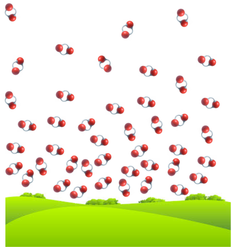
At a conceptual level, this is actually a pretty simple problem of balancing kinetic and potential energy. Imagine following the trajectory of a single air molecule (say, an oxygen molecule) for a long time. This molecule moves in a sort of random trajectory, buffeted about by other air molecules, and it rises and falls in altitude. As it does so, it trades some of its kinetic energy for gravitational potential energy when it rises, and then trades that potential back for kinetic energy when it falls. If you average the kinetic and potential energy of the molecule over a long time, you’ll find that they are similar in magnitude, in just the same way that they would be for a ball that bounces up and down over and over again.

There is actually an important and precise statement of this equality, called the virial theorem, which in our case says that

$2 \langle \textrm{K.E.}_z \rangle = \langle \textrm{P.E.} \rangle$

where $\langle \textrm{K.E.}_z \rangle$ is the average ~~potential~~ kinetic energy in the vertical direction and $\langle \textrm{P.E.} \rangle$ is the average potential energy.

The gravitational potential energy of a particle of mass $m$ is just

$\textrm{P.E.} = mgh$

and the typical kinetic energy of the air molecule is related to the temperature, (this is, in fact, the definition of temperature):

$\langle \textrm{K.E.}_z \rangle = \frac{1}{2} k_B T$ ,

where $k_B$ is Boltzmann’s constant and $T$ is the absolute temperature (i.e., measured from absolute zero). On the earth’s surface, $k_B T$ is about 25 milli-electronvolts, or $\approx 4 \times 10^{-21}$ Joules.

Using these equations to solve for $h$ gives $h \sim k_B T /(m g)$ , which is about 5 miles.

Everything makes sense so far, but let’s ask a more interesting question: What is the function that describes how the thickness of the atmosphere decays with altitude? In other words, what is the probability density $p(z)$ for a given air molecule to be at altitude $z$ ?

Pastoral scene, with oxygen molecules

Let’s take a God-like perspective on this question [insert joke here about typical physicist arrogance]. Imagine that you could choose some function $p(z)$ from the space of all possible functions, and in order to make your choice you must first ask the question: which function is best?

“Best” may seem like a completely subjective word, but in physics we often have optimization principles that let us define the “best solution” in a very specific way. In this case, the best solution is the one with the highest entropy. Remember that saying “this state has maximum entropy” literally means “this state is the one with the most possible ways of happening”. 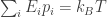So what we are really searching for is the function $p(z)$ that is most probable to appear from a random process.

The entropy of a probability distribution $p(z)$ is

$S = - k_B \int_0^\infty p(z) \ln p(z) dz$ ,

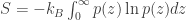
This is a generalization of the Boltzmann entropy formula $S = k_B \ln W$ (which is a sufficiently big deal that Boltzmann had it engraved on his tombstone).

Now, there are two relevant constraints on the function $p(z)$ . First, it must be normalized:

$\int_0^\infty p(z) dz = 1$ .

Otherwise, it wouldn’t be a proper probability distribution.

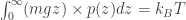
Second, the distribution must correspond to a finite average energy. In particular, the average potential energy of an air molecule must be $k_B T$ . Since the energy of a molecule with altitude $z$ is $m g z$ , we have the second constraint

$\int_0^\infty (m g z) \times p(z) dz = k_B T$ .

Now, for those of you who read the previous post, this kind of problem should start to look familiar. To recap, we want

a function $p(z)$ that maximizes some quantity $S$
and is subject to two constraints

This is a job for Lagrange multipliers!

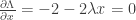
To optimize the quantity $S$ using Lagrange multipliers, we start by writing the Lagrange function

$\Lambda = S - \lambda_1 [\int_0^\infty p(z) dz - 1] - \lambda_2 [mg \int_0^\infty z p(z) dz - k_B T]$ .

Here, the two quantities in brackets represent the constraints. Putting in the expression for $S$ and then taking the derivative $\partial \Lambda/\partial p$ and setting it equal to zero gives

$-k_B [\ln p(z) + 1] - \lambda_1 - \lambda_2 m g z = 0$

Since $p$ appears only in a logarithm, rearranging and solving for $p(z)$ gives something like

$p(z) = \textrm{const.} \times e^{-\textrm{const.} \times z}$

Now we can use the two constraint (normalization and having a fixed expectation value of the energy) to solve for the values of the two constants. This procedure gives

$p(z) = \frac{1}{h} e^{-z/h}$ ,

where $h = k_B T /(m g)$ is the same “typical thickness” that we estimated at the beginning.

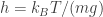
Maybe this seems like a funny little exercise in calculus to you, but what we just did is actually a big deal. We started with very little knowledge of the system at hand: we didn’t know anything about the composition of Earth’s atmosphere, or how air molecules collide with each other, or any principles of physics at all except for the high-school level formula for gravitational potential energy and the understanding that temperature is a measure of kinetic energy. But that was enough to figure out the precise formula for atmospheric density, just by demanding that such a formula must be the most likely one, in the sense of having the highest entropy.

And, it turns out, our derivation is pretty good. Here’s data from the Naval Research Laboratory:

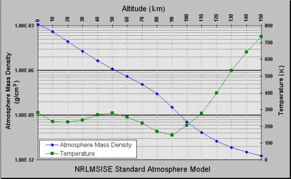
Notice that the density of the atmosphere looks very much like an exponential decay (a straight line on this plot) up until about 80 km of altitude. At higher altitude there’s a sort of crazy increase in temperature (probably due to direct heating from solar radiation and an absence of equilibration with the thicker atmosphere below it) that slows down the decay of atmosphere density.

The Boltzmann Distribution

With a relatively small amount of work, we figured out how thick Earth’s atmosphere is, and how the that thickness depends on altitude.

But it turns out that what we really just did is something much bigger. We found a way to relate energy — in that last problem, expressed through altitude — to probability.

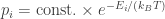
So let’s take a step back, and look over what we did while thinking of a much bigger, more general problem. Suppose that some system (it could be a single particle, or it could be a set of many particles) has many different configurations that it can take. Let’s say, generically, that the energy of some configuration $i$ has energy $E_i$ . Now let’s ask: what is the best probability distribution $p_i$ for describing how likely each configuration is?

Despite knowing literally nothing about the specifics of this problem, we can still approach it in exactly the same way as the last one. We say that the distribution $p_i$ must maximize the entropy:

$S = - \sum_i p_i \ln p_i$ ,

while it is subject to the normalization constraint

$\sum_i p_i = 1$

and the constraint of having a finite average energy $k_B T$ :

$\sum_i E_i p_i = k_B T$ .

These equations all look identical to the ones we wrote down when talking about the atmosphere. So you can more or less just write down the answer now by looking at the previous one, without doing any work:

$p_i = \textrm{const.} \times e^{-E_i/(k_BT)}$ .

Now this formula is a really big deal. It is called the Boltzmann distribution.

The Boltzmann distribution allows you, very generically, to say how likely some outcome is based only on its energy. The only real assumption behind it is that the system has time to evolve in a sort of random way that explores many possibilities, and that its average quantities are not changing in time. (This set of conditions is what defines equilibrium.)

It’s a formula that rears its head over and over in physics, turning seemingly impossible problems into easy ones, where all the details don’t matter. I’m pretty confident that, if I had discovered it, I would put it on my tombstone also.

Footnote:

While I, personally, have used the Boltzmann formula countless times in my life, my favorite application of it was to study pedestrian crowds. It turns out that humans have a very well-defined analogue of “interaction energy” with each other that dictates how they move through crowds. The Boltzmann distribution is what enabled us to figure out how that interaction worked!

More people should know about Lagrange multipliers

July 6, 2018

by Brian

One of the most useful concepts I learned during my first year of graduate school was the method of Lagrange multipliers. This is something that can seem at first like an obscure or technical piece of esoterica – I had never even heard of Lagrange multipliers during my undergraduate physics major, and I would guess that most people with technical degrees similarly don’t encounter them. When I was first taught Lagrange multipliers, my reaction was something like “okay, I’m guessing this is just a mathematical trick used by specialists in a few specific circumstances. After all, I’ve done just fine without it so far.”

But, like many mathematical tools, Lagrange multipliers are one of those things that open doors for you. Once you understand how to do optimization using them, whole worlds of problems open up that you would have previously thought were too hard, or had no good solution. I personally have found myself using Lagrange multipliers for everything from statistics to quantum mechanics, from electron gases to basketball.

My goal for the next few posts is to derive some of the most important equations in physics: the “distribution functions” that relate energy to probability. But before we get there it’s worth pausing to appreciate the power of Lagrange multipliers, which will be one of the major tools that enable us to understand how nature maximizes probability.

A simple example

The basic use of Lagrange multipliers is fairly simple: they are used to find the maximum or minimum of some function in situations where you have constraints. For example, the standard introductory problem to Lagrange multipliers is usually something like this:

Suppose that you are living on an inclined plane described by the equation z = -2x + y, but you can only move along the circle described by x² + y² = 1. What is the highest point (largest z) that you can reach? What is the lowest point?

plane_with_circle

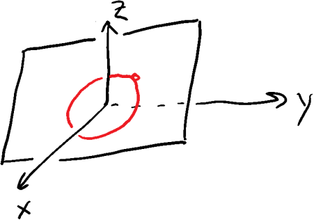
What makes this problem tricky, of course, is the relationship between x and y. If x and y were independent of each other, then you could simply maximize the function with respect to each variable independently. But the constraint that x² + y² = 1 means that you have to work harder.

If you haven’t learned the method of Lagrange multipliers, your first instinct will probably be to try and reduce the number of variables in the problem. For example, you could try to use the constraint equation x² + y² = 1 to solve for y in terms of x, and then plug the solution for y into the equation that you’re trying to maximize or minimize. Then you can hope to get the maximum or minimum by taking the derivative of z with respect to your one remaining variable, x. If you try this method, however, you’ll find that it gets messy really quickly. And heaven help you if you have a problem with many variables or many constraints – you’ll have to do a whole lot of messy solving and substituting before you get the equation down to a single variable.

The key idea behind the method of Lagrange multipliers is that, instead of trying to reduce the number of variables, you increase the number of variables by adding a set of unknown constants (called Lagrange multipliers). What you get in exchange for increasing the number of variables, however, is a new function (commonly denoted Λ), for which all the variables are independent. With this magic new function you can do the optimization simply by taking the derivative of Λ with respect to each variable one at a time. This function (called the Lagrange function) is:

$\Lambda(x,y, ..., \lambda_1, \lambda_2 ...) = (\textrm{function you're trying to optimize}) ...$

$- \lambda_1 (\textrm{first constraint equation}) - \lambda_2 (\textrm{second constraint equation}) - ...$

[Here when I write “constraint equation”, I really mean “the left-hand side of a constraint equation, written so that the right-hand side is zero”.] You can find the maximum or minimum of this function by setting all of its derivatives to zero:

$\frac{\partial \Lambda}{\partial x} = \frac{\partial \Lambda}{\partial y} = ... = \frac{\partial \Lambda}{\partial \lambda_1} = \frac{\partial \Lambda}{\partial \lambda_2} = ... = 0$

So in our example problem, the Lagrange function is

$\Lambda = -2x + y - \lambda(x^2 + y^2 - 1)$ .

The first part, $-2x + y$ , is the function z that we’re trying to maximize/minimize, and the part in parentheses, ( $x^2 + y^2 -1$ ), is the constraint. The three equations that come from taking the derivatives of are

$\frac{\partial \Lambda}{\partial x} = -2 -2 \lambda x = 0$

$\frac{\partial \Lambda}{\partial y} = 1 - 2 \lambda y = 0$

$\frac{\partial \Lambda}{\partial \lambda} = x^2 + y^2 - 1 = 0$ .

This last equation is just a repetition of the constraint equation, but the other two are really useful. You can manipulate them pretty easily to find that

Using the constraint equation allows you to solve for $\lambda$ , and after a relatively painless bit of plugging and chugging you’ll arrive at two solutions:

$x = -2/\sqrt{5}$ , $y = 1/\sqrt{5}$ , $z = \sqrt{5}$

$x = 2/\sqrt{5}$ , $y = -1/\sqrt{5}$ , $z = -\sqrt{5}$ .

These are the maximum and the minimum that we’re looking for.

Not bad, right?

The real power of Lagrange multipliers

What’s really great about Lagrange multipliers is not that they can solve rinky-dink little problems like the one above, where you’re looking for the best point on some function. What’s amazing is that Lagrange multipliers can find you an optimal function.

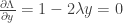
Let’s imagine, as an example, the following contrived problem. Suppose that there is an outdoor, open-air rock concert, and music fans crowd around the stage to hear. In general, the density of the crowd will be highest right next to the stage, and the density will get lower as you move away.

In choosing where to stand, the audience members have to weigh the tradeoff between their desire to be close to the band and their desire to avoid a very dense crowd. Suppose that there is some “happiness function” that weighs both of these factors together. For the purposes of our contrived example, let’s say it’s

$h = \frac{1}{1+x} - c \rho^2$ .

Here, h is the happiness of a person at a distance x (in some units) from the stage, c is some constant, and $\rho$ is the density of the crowd around them. The term $1/(1+x)$ is supposed to represent the enjoyment that people get from being close to the band, which decays as you move away, while the negative term represents a person’s discomfort at being in an extremely dense crowd. The interesting question is: what distribution of crowd density, $\rho(x)$ , maximizes the total happiness of everyone at the concert? In other words, what is the very best function $\rho(x)$ ?

While h(x) represents the happiness of a particular person at position x, the total happiness of everyone in the crowd is

$H = \int h(x) \rho(x) dx$ .

That is, H is equal to the number of people $\rho(x) dx$ in any small interval $(x, x+dx)$ of position, multiplied by the happiness of those people, and summed over all positions. This is the function that we will try to maximize.

The constraint on this function is that there is some fixed total number N of people in the crowd:

$\int \rho(x) dx = N$ .

Now, using the recipe outlined above, we can write down a Lagrange function

$\Lambda = H - \lambda ( \int \rho(x) dx - N)$ .

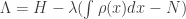
In the previous problem, we were only trying to find optimal values of two specific variables: x and y. Here, we are trying to find the optimal value of $\rho(x)$ at every value of x. So you can think that our goal is to optimize the function $H$ with respect to infinitely many variables: one value of for every possible position. Beyond that conceptual generalization, however, the recipe for solving the problem is the same. If it helps, you can imagine dividing up the set of all possible positions into discrete points: $x_1, x_2, x_3$ , etc. Each position $x_i$ has a corresponding value of $\rho_i$ and a corresponding value of the local happiness function $h_i = 1/(1+x_i) - c \rho_i^2$ . The function to be optimized is then just

$H = h_1 \rho_1 + h_2 \rho_2 + ...$

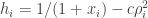
while the constraint condition is

$\rho_1 + \rho_2 + ... = N$ .

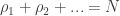
The optimality of the Lagrange function says that

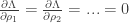
$\frac{\partial \Lambda}{\partial \rho_1} = \frac{\partial \Lambda}{\partial \rho_2} = ... = 0$

Let’s consider some particular point $\rho_i$ . The Lagrange equation

$\frac{\partial \Lambda}{\partial \rho_i} = 0$

gives

$\frac{\partial}{\partial \rho_i} (h_i \rho_i) - \lambda = 0$

$\frac{1}{1 + x_i} - 3 c \rho_i^2 - \lambda = 0$ .

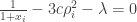
Drop the subscript i, and you’ll see that this equation is actually telling you about the functional dependence of the density on the position x. In particular, solving for $\rho$ gives

$\rho(x) = \sqrt{ \frac{1}{3c} ( \frac{1}{1 + x} - \lambda) }$ .

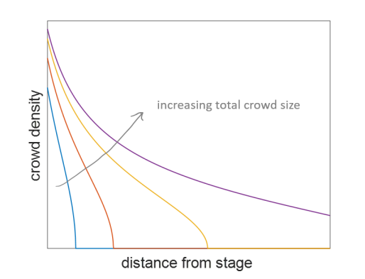
The value of $\lambda$ depends on the number of people N in the crowd – a larger crowd means $\lambda$ gets closer to zero. You can go back and solve for its value by doing the integral of $\rho(x)$ , but in the interest of not being too pedantic I’ll spare you the details. The final solution for $\rho(x)$ looks something like this:

rock_concert_density

The takeaway from this funny exercise is that Lagrange multipliers allow you to solve not just for the optimal point on some function, but for the optimal kind of function for some environment. This is the kind of problem that I didn’t even realize was well-posed until I got to graduate school, and the ability to solve such problems is an extremely powerful tool in physics. Indeed, it is one of the recurring themes of physics that when we want to know which laws govern nature, we start by asking “which laws would give the smallest (or largest) total amount of X?”

When it comes to asking those kinds of questions, Lagrange multipliers are like a math superpower.

UPDATE:

A couple people have commented (on Twitter) that there is a simple pictorial way to think about Lagrange multipliers and why they work, and there’s no reason for me to make them seem like black magic. This is true, of course, so let me try and give a quick recap of the intuitive explanation for the method.

Consider the first example in this post, where you are constrained to move along the circle $x^2 + y^2 = 1$ . Imagine an arrow pointing in the direction of your motion as you walk around the circle. And now imagine also an arrow that represents the gradient of the function $f$ you are trying to maximize (remember, the gradient of a function points in the direction of greatest increase of that function). If the arrow for the direction of your motion points in the same direction as the gradient, then you are moving directly uphill. If the arrow of your motion points in the opposite direction as the gradient, then you are moving directly downhill.

Most of the time, there will be some particular angle between the direction of your motion and the gradient. This means you are moving “somewhat uphill” or “somewhat downhill”. But at the very peak height (or at the very lowest point) of your trajectory, your motion will be exactly perpendicular to the gradient, meaning that for that instant you are moving neither uphill nor downhill.

The key idea is to imagine a function $g(x,y)$ that represents the constraint — in our example $g(x,y) = x^2 + y^2 - 1$ . The constraint (the definition of the circle you are constrained to walk along) represents the contour $g(x,y) = 0$ . The gradient of the function $g(x,y)$ always points perpendicular to the direction of your motion along the circle, since by definition moving along the circle does not increase the value of $g(x,y)$ .

So, putting all the pieces together, we arrive at the conclusion that at a maximum or minimum, the gradient of $f$ points parallel to the gradient of $g$ .

In equation form, this is

$\partial_{x} f = \lambda \partial_{x} g$ ,

$\partial_{y} f = \lambda \partial_{y} g$ ,

…

where $\lambda$ is some constant.

This is exactly the Lagrange multiplier equation $\partial_{x} \Lambda = \partial_{y} \Lambda = ... = 0$ , with $\Lambda = f - \lambda g$ .

If this all still feels pretty opaque, there is a very nice video series from Khan academy on this subject.

Squiggle reasoning: the skydiving animals problem

October 20, 2016

by Brian

There is a common conception that physics is a business of writing and solving exact equations. This idea is not untrue, in the sense that physicists generally prefer to produce exact solutions when they can. But precise equations can be slow: they are often cumbersome to work with and can obscure important concepts with a tedium of error-checking and term-collecting. For these reasons, physicists often figure things out (at least in the initial stages of problem solving) using a kind of semiquantitative reasoning that doesn’t make use of exact equalities.

In this kind of reasoning, all (or most) equations are downgraded from having an equals sign, $A = B$ , which means “A is equal to B”, to having a “squiggle” sign, $A \sim B$ , which means “A is equal to B up to some numeric factor that I don’t particularly care about.”

This may seem kind of dumb to you. Why reason with squiggles when you can write exact equations instead? But the truth is that “squiggle reasoning” often allows you to figure things out much more quickly and easily than you would ever be able to if you insisted on writing only exact equations. And as long as you are willing to live with some ignorance about exact numerical values, you sacrifice very little in terms of conceptual clarity.

As it happens, I designed and taught a short course last year for high school students that introduces basic ideas in quantum mechanics using squiggle reasoning. (I am teaching the course again this year.) As an introduction, I gave the students the following problem:

If a bunch of animals of different sizes all jump out of an airplane together, how fast do they each fall?

In this post I’ll take you through the answer to this problem, which can perhaps serve as a gentle introduction to quantitative reasoning in situations where you don’t know how to (or don’t want to) write down exact equations.

Gravitational Force

The starting point in solving this problem is to forget that animals have particular shapes. That is, simplify the geometry of a given animal down to a single number: its “size” $L$ . Now, obviously for any real animal you will get a different number for the “size” depending on which direction you choose for the measurement. For example, I personally am something like 1.8 meters tall, 0.6 meters wide, and 0.3 meters thick. But if you just want a number that is in the right ballpark, it is fair to say that I am ~1 meter in size, as opposed to 1 centimeter or 1 kilometer.

To connect to an old trope, this kind of thinking isn’t really “assuming a cow is a sphere” so much as it is “not caring about the difference between a cow and a sphere”.

cow

Now you can ask: what is the force of gravity acting on an animal of size 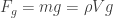$L$ ? Well, the force of gravity is $F_g = m g = \rho V g$ , where $g \approx 10 \textrm{ m/s}^2$ is the acceleration due to gravity, $m = \rho V$ is the animal’s mass, $\rho$ is the density of the animal, and $V$ is its volume.

Since we have decided to forget about all specifics of the animal’s shape, making an estimate for the animal’s volume is actually very easy:

$V \sim L^3$ .

In fact, in squiggle reasoning, every three-dimensional shape has volume $\sim (\textrm{size})^3$ , unless you have decided to look at some shape that is especially long and skinny. This means that we can easily write an approximate equation for the force of gravity acting on the animal:

$F_g \sim \rho g L^3$ .

Drag force

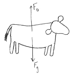
Immediately after jumping out of the airplane, the $L$ -sized animal in question is in freefall, and accelerates downward at a rate $\sim g$ . However, after falling for a little while its acceleration is halted by the force of all the air rushing back against it. The animal will eventually reach a steady downward velocity determined by the two forces being in balance:

freebody

So how big is the drag force $F_D$ ?

Of course, the exact answer to this question depends on the shape of the animal. If you really wanted to know, with numeric accuracy, the value of the drag force, then you would need to understand the air flow pattern around the animal. This would presumably require you to stick the animal in a wind tunnel and make careful measurements. (And you would get different answers depending on which way the animal was facing).

But at the level of squiggle reasoning, we can figure out the drag force using a simple thought exercise. Imagine the process of throwing a big block of air at the animal:

This block is taken to have the same cross-sectional size as the animal (area $L^2$ ) , and some length $w$ . The mass of the air block is therefore something like $m_\textrm{air} \sim \rho_\textrm{air} L^2 w$ . If the block is thrown with a speed $v$ , then it has a kinetic energy $KE \sim m_\textrm{air} v^2 \sim \rho_\textrm{air} v^2 L^2 w$ . (I’m sure you learned that first equation as $KE = \frac{1}{2} mv^2$ , but when you’re doing squiggle reasoning there’s no reason to fuss about $\frac{1}{2}$ ’s.)

In order to stop the block of air, the animal applies a force that does work on the block equal to $KE$ . The work is equal to the drag force of the air multiplied by the distance over which the force is applied. That distance is $\sim w$ ; you can think that the force is applied continuously as the air block smooshes into the animal’s side. Thus, we have $F_D w \sim KE$ , and therefore

$F_D \sim \rho_\textrm{air} v^2 L^2$ .

Of course, when the animal is falling through the air, this drag force is applied continuously, as the animal finds itself continuously colliding with “blocks of air” that move toward it with speed $v$ .

Final Answer: never skydive in the rain

Now we are ready to get an answer: equating $F_g$ with $F_D$ and solving for $v$ gives us

$v \sim \sqrt{\rho g L / \rho_\textrm{air}}$ .

Thus we arrive very quickly at an important semi-quantitative conclusion: larger animals fall faster, with a terminal velocity that grows as the square root of the animal’s size.

In fact, you can use this equation to get a pretty good order-of-magnitude estimate for the terminal velocity $v$ , using the fact that pretty much all animals have the same density as water, $\rho \sim 1 \textrm{ g/cm}^3$ , while air is about 1000 times less dense.

In particular, the squiggle equation for $v$ suggests that a meter-sized human has a terminal velocity on the order of $\sim 100 \textrm{ m/s}$ . (For reference, one m/s is about 2 mph — within the accuracy of our squiggle reasoning you can take a meter-per-second and mile-per-hour to be roughly the same thing.) A centimeter-sized cockroach has a terminal velocity of $\sim 10 \textrm{ m/s}$ , and a 10-meter-sized whale falls at about $300 \textrm{ m/s}$ ; three times faster than you do.

Thus, you can see pretty quickly why falling off a building is deadly for you (hitting the ground at ~ 100 mph is worse than just about any car accident) but not deadly for insects (hitting the ground at a couple mph is no big deal).

In fact, there is a pretty practical implication of this result (besides “don’t fall off a building”): You should never go skydiving in the rain. You might think (as I initially did) that it would be a sort of magical and pleasant experience, wherein you fall together with the raindrops like an astronaut playing with zero-gravity water droplets. But the truth is much more unpleasant: the meter-sized you will be falling at ~1o0 mph, while the millimeter-sized raindrops fall at a slow ~3 mph. So, from your perspective, you’ll be getting stabbed by raindrops that blast you in the face at ~97 mph.

Highly unpleasant, and just a small amount of squiggle reasoning before you jump can save you the trouble.

Toward a culture of tolerating ignorance

June 13, 2016

by Brian

Lately I have seen an increasingly honest, and increasingly public discussion about the feelings of inadequacy that come with trying to be a scientist.

For example, here Anshul Kogar writes about the “Crises in Confidence” that almost invariably come with trying to do a PhD.

In this really terrific account, Inna Vishik tells the story of her PhD in physics, and the various emotional phases that come with it: from “hubris” to “feeling like a fraud”.

I might as well add my own brief admissions to this discussion:

More or less every day, I struggle with feeling like I am insufficiently intelligent, insufficiently hardworking, and insufficiently creative to be a physicist.
These feelings have persisted since the beginning of my undergraduate years, and I expect them to continue in some form or another throughout the remainder of my career.
I often feel like what few successes I’ve had were mostly due to luck, or that I “tricked” people into believing that I was better than I actually am.

I have gradually come to understand that these kinds of feelings, as dramatic as they seem, are relatively normal. Some degree of impostor syndrome seems to be the norm in a world where intellect is (purportedly) everything, and where you are constantly required to “sell” your work. And I should probably make clear that I am not a person who lacks for confidence, in general. (If you asked my wife, she might even tell you that I am an unusually, perhaps frustratingly, confident person.)

I have also come to understand that there is a place for a person like me in the scientific enterprise. I have very real shortcomings as a scientist, both in talent and in temperament. But everyone has shortcomings, and in science there is room for a great variety of ability and disposition.

There is one practice that I have found very helpful in my pursuit of a scientific career, and which I think is worth mentioning. It’s what I call fostering a “culture of tolerating ignorance.”

Let me explain.

As a young (or even old) scientist, you continually feel embarrassed by the huge weight of things you don’t know or don’t understand. Taking place all around you, among your colleagues, superiors, and even your students, are conversations about technical topics and ideas that you don’t understand or never learned. And you will likely feel ashamed of your lack of knowledge. You will experience some element of feeling like a fraud, like someone who hasn’t studied hard enough or learned quickly enough. You will compare yourself, internally, to the sharpest minds around you, and you will wonder how you were allowed to have the same profession as them.

These kinds of feelings can kill you, and you need to find a way of dealing with them.

I have found that the best strategy is to free yourself to openly admit your ignorance. Embrace the idea that all of us are awash in embarrassing levels of ignorance, and the quickest way to improve the situation is to admit your ignorance and find someone to teach you.

In particular, when some discussion is going on about a topic that you don’t understand, you should feel free to just admit that you don’t understand and ask someone to explain it to you.

If you find yourself on the other side of the conversation, and someone makes such an admission and request, there are only two acceptable responses:

Admit that you, also, don’t understand it very well.
Explain the topic as best as you can.

Most commonly, your response will be some combination of 1 and 2. You will be able to explain some parts of the idea, and you will have to admit that there are other parts that you don’t understand well enough to explain. But between the two of you (or, even better, a larger group) you will quickly start filling in the gaps in each others’ knowledge.

A culture where these kinds of discussions can take place is a truly wonderful thing to be a part of. In such an environment you feel accepted and enthusiastic, and you feel yourself learning and improving very quickly. It is also common for creative or insightful ideas to be generated in these kinds of discussions. To me, a culture of tolerating ignorance is almost essential for enjoying my job as a scientist.

The enemies of this kind of ideal culture are shame and scorn. The absolute worst way to respond to someone’s profession (or demonstration) of ignorance is to act incredulous that the person doesn’t know the idea already, and to assert that the question is obvious, trivial, and should have been learned a long time ago. (And, of course, someone who responds this way almost never goes on to give a useful explanation.) An environment where people respond this way is completely toxic to scientific work, and it is, sadly, very common. My suggestion if you find yourself in such an environment to avoid the people who produce it, and to instead seek out the company of people with whom you can maintain enthusiastic and non-scornful conversations.

I have personally benefited enormously from those kinds of people and that kind of culture. At this point in my career, I would hope that I could tolerate a colleague admitting essentially any level of scientific ignorance, and that I would respond with a friendly explanation of how I think about the topic and a declaration of the limits of my own understanding.

As I see it, ignorance to essentially any degree is not a crime. There is simply too much to know, and too many perspectives from which each idea can be understood, to shame someone for admitting to ignorance. The only crime is professing to understand something that you don’t, or making claims that are not supported by your own limited understanding.

Good enough for me

April 16, 2016

tags: Virginia Tech

by Brian

Today, April 16, is the one day in the year when I use this blog for very personal purposes. In particular, I reserve the day for remembering Virginia Tech and my time there. (Past years’ writings are here: 1, 2, 3, 4, 5).

If you’re here for physics-related content, just hold on; a new post should be up within a few days.

On the afternoon of May 12, 2007, I almost did something terrible.

That particular Saturday was the day of my college graduation. The physics department was holding a warm and enthusiastic ceremony for the seventeen of us who were graduating, with plenty of food and lots of cheer spread among the hundred or so people in attendance.

The dangerous part was that our valedictorian was an unusually generous person, and had offered to split the valedictory speech with me. I probably should have declined, but I was apparently neither sufficiently polite nor sufficiently humble to do so. And so I was slated to give a short speech as part of the ceremony.

What made this dangerous was that late April and early May of 2007 were confusing times for those of us at Virginia Tech. During the week or so before the ceremony, as I sat down to try and draft my graduation speech, I found that I kept coming back to the themes we were all facing after the Virginia Tech shooting: loss, grief, anxiety, community, etc.

With those themes ever-present in my mind, I wrote something that was predictably awful. Most of the specifics of what I wrote have been (graciously) lost to my memory, but you can probably imagine it easily enough: a painfully over-earnest speech that betrayed a deficit of self-awareness. It would have been the sort of thing that drips with a sense of how moved the speaker is by himself.

To this day I still have nightmares where I find that I have become like “Mike”, the guy who threw me into an unreasonable rage by writing a terrible poem. I guess I almost did the same thing.

But a very fortunate thing happened to me on the morning of Saturday, May 12:
I woke up feeling happy.

As it so happens, on the day of my graduation, surrounded by my family members and friends, I was happy. I wasn’t “confused” or fragile or maudlin. It was much more simple. I was just happy.

And so I made the fortunate decision to ditch that terrible speech in favor of something more straightforward.

I decided to sing a song.

During college I had actually made a minor habit of writing parody songs about being a physics major and about the VT physics department. So I guess I was sufficiently well-practiced to be able to put together a song pretty quickly, in time for the ceremony.

The lyrics are reproduced below.

Now, I should probably warn you in advance that this is not a good song. It’s full of overzealous dorkiness and now-incomprehensible inside jokes. But I treasure the memory of standing in front of that audience and singing this song. Because it is a memory of being happy; of feeling yourself surrounded by people who like you and care about you; and of being unashamed of who you are, and unafraid of the future.

I should mention, by the way, that our valedictorian’s half of the speech was awesome. It was more or less entirely made up of jokes and impressions of our professors, and the whole afternoon was baked in geekish enthusiasm.

Good enough for me

A song for the Virginia Tech physics class of 2007

[sung to the tune of “Me and Bobby McGee”, as performed, for example, by Janis Joplin]

Standing in my cap and gown
waiting to hear my name
I’m feeling near as divided as a triplet state.
So many things I never learned,
so many tests where I got burned,
but at least I beat the high physics dropout rate.

Well my education has served me well.
It taught me some important skills,
and it taught me to avoid what I can’t do.
From Tauber’s quantum purgatory
to Mizutani’s rambling stories
I’ve mislearned more science than most people ever knew.

Well a diploma’s just a way of saying
“you’re good enough to leave
but hey, we’re not making any guarantees.”
And I may never solve a single problem
in a rotating reference frame…
But inertial frames are good enough for me.
Good enough for me to get my degree.

From the sub-basement physics lounge
to our campouts in the woods
just think of all the nerdy things we’ve done.
Text Twist games that last for months,
telling awful science puns,
yeah we’ve invented a language of our own.

Some of us can obfuscate with pictures,
but all of us speak math,
And if you say it sounds like Greek,
then I’ll have to agree.
And while we may sound pretty smart,
I’ll tell you a secret truth:
none of us know what quantum mechanics means.

Well a diploma’s just a way of saying
“you’re good enough to leave
no matter what score you got on the GRE.”
I may not know how to solve the time-dependent Schrodinger equation…
But time-independent is good enough for me.
Good enough for me to get my degree.

Well a diploma’s just a way of saying
“you’re good enough to leave
but if you want respect you’ll still need a PhD.”
And though my time here has seemed short
and it’s hard for me to leave…
Well, I guess five years were good enough for me.
Good enough for me to get my degree.

good_enough

surveyor

February 15, 2016

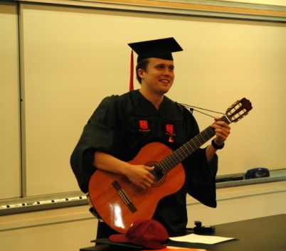
tags: fractal dimension, Michael Keaton, Pictures for Sad Children, surveyor, the smallest one is michael

by Brian

There used to exist a really wonderful webcomic called Pictures for Sad Children. A few years ago its creator, John Campbell, grew tired of the project and removed all of it from the internet. But the comic was hugely influential, and you can find most of its pieces reproduced online if you do a Google search.

Lesser known is the author’s smaller follow-up comic that was (somewhat bizarrely) themed around a fictionalized recounting of the life of the actor Michael Keaton. This comic has also been taken down completely, and it is much harder to find any of its pieces online.

There was one of the Michael Keaton comics that I loved in particular, though, and which I managed to find using a lot of patience and the Internet Archive site. I am reproducing it here not because I have any right to do so, but because it was too sad for me to think that it might get lost to humanity.

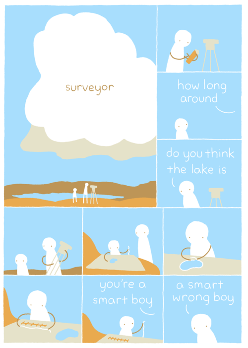
tumblr_mj90gz0Kv81rngbhio1_500 tumblr_mj90hkGYKz1rngbhio1_500 tumblr_mjaovmGylb1rngbhio1_r3_500

Game theory of vaccination

February 9, 2016

tags: game theory, MMR, vaccination

by Brian

How unreasonable is it to not vaccinate your children?

I ask this not as a rhetorical question, but as a mathematical one. How do we describe, mathematically, the benefits and risks of vaccination? What does this description tell us about the reasonableness (or unreasonableness) of not vaccinating?

These days, most of the debate about vaccination is centered around questions of misinformation, misunderstanding, delusion, and conspiracy. But all this shouting obscures an interesting and very real mathematical question.

So let’s consider the dilemma of a perfectly well-informed and perfectly rational person faced with the decision of whether to vaccinate their child against some particular disease. Making this decision involves weighing issues of risk and reward, and thinking about selfishness and altruism.

Luckily for us, there is an entire mathematical science devoted to addressing these kinds of questions: the science of Game Theory.

In this post I want to take a game-theoretical look at the problem of vaccination. In particular, we’ll ask the questions: under what conditions is a disease dangerous enough that you should vaccinate? And is doing what’s best for your child different from doing what’s best for society as a whole?

kid_shot

Risk and Reward

The key idea in this analysis is as follows. When you vaccinate your child, you provide them with the benefit of immunity against a disease that they might encounter in the future. This benefit is potentially enormous, and life-saving.

However, if your child lives in a population where nearly everyone already has the vaccine, then the benefit of the vaccine to your child is greatly reduced. After all, if everyone around is effectively immune to the disease already, then the group’s “herd immunity” will greatly reduce the chance that your child ever gets exposed to the disease in the first place.

You might therefore be tempted to decide that even a very small risk inherent in the vaccine would make it not worthwhile. And, certainly, such risks do exist. For example, there is a very small chance that your child could have a serious allergic reaction to the vaccine, and this reaction could lead to things like deafness or permanent brain damage. If your child is already getting “herd immunity” from everyone else’s vaccination anyway, then why risk it?

Let’s consider this question in two steps. First, we’ll ask what is the optimal vaccination rate. This is the rate that maximizes the safety and well-being of the whole population. Then, we’ll ask the more pointed question: which is the decision that is best for your child alone, given that as a parent your concern is to minimize the chance of harm to your child, and not to the world as a whole.

Let’s discuss these ideas in a completely theoretical sense first, and then we’ll put some numbers to them to see how the real world compares to the theoretical ideal.

The optimal behavior

Imagine, first, a population where everyone is vaccinated against a particular disease except for some fraction x of non-vaccinators. Now suppose that a randomly-chosen individual gets exposed to the disease.

If the vaccine is highly effective, then the chance that this person will contract the disease is the same as the chance that they are not vaccinated: x. In the event that this person does contract the disease, then they will expose some number n of additional people to the disease. This wave of second-hand exposures will lead to a wave of third-hand exposures, and so on. At each wave there is a multiplication by n in the number of potentially exposed people, and a (hopefully small) probability x of the disease being communicated.

You can diagram the spread of the disease something like this:

epidemic

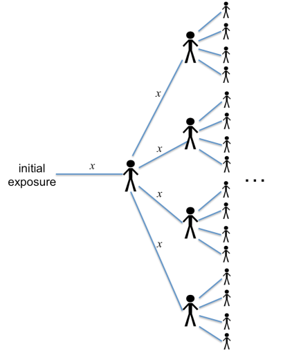
This picture illustrates the case n = 4 (i.e., every infected person exposes an average of four other people). Each branch labeled “x” shows the probability of the disease being spread at that step.

If you add up the expected number of infected people, you’ll get

$(\text{total infected}) = x( 1 + n x (1 + nx(1 + ... ) ) )$

$(\text{total infected}) = x \sum_{i = 0}^{\infty} (n x)^i$

$(\text{total infected}) = x/(1 - n x)$

This last equation already suggests an important conclusion. Notice that if the rate of non-vaccination, x, gets large enough that $n x \geq 1$ , then the total number of infected people blows up (it goes to infinity).

In other words, if $n x \geq 1$ then the population is susceptible to epidemics. There is a very simple way to interpret this condition: $n x$ is the average number of new people to whom a given sick person will pass their infection. If each sick person gets more than one other person sick, then the disease will keep spreading and you’ll get an epidemic.

If this condition is met, then there is no question about vaccinating. A population that is susceptible to epidemics is one where you need to get vaccinated. End of story.

But let’s assume that you live somewhere where this particular disease doesn’t cause epidemics anymore. (Like, say, mumps in the USA – more on this example below.) An absence of epidemics generally implies $n x < 1$ , and any flare-up in the disease will be relatively small before it dies off.

Let’s say that every so often someone within the population is exposed to the disease. We’ll call this the rate of exposure, E, which can be defined as the number of initial exposures in the population per year. Combining this rate with the equation above means that

$E x/(1 - n x)$

people will be infected per year.

This rate of disease-induced sickness should be compared with the rate of vaccine-induced sickness. If a fraction x of people are not vaccinated, that means that $N (1- x)$ people do get vaccinated, where $N$ is the total number of people in the population. As a yearly rate, $N(1-x)/T$ people are vaccinated per year, where $T$ is the average lifetime of a person (or, if the vaccine requires periodic boosters, $T$ is the time between successive vaccinations). Let’s suppose, further, that the vaccine makes a child sick with some probability $v$ .

What this all means is that there are

$(1-x) N v/T$

vaccine-induced illnesses in the population every year.

(If you’re getting lost keeping track of all these variable names, don’t worry. Only two will matter in the end.)

From a population-wide standpoint, the optimal rate of vaccination is the one that minimizes the total amount of illness in the population per year:

$F = E x/(1 - nx) + (1-x) N v/T$ .

Taking the derivative $dF/dx$ of the function $F$ and setting it equal to zero gives a solution for the optimal non-vaccination rate:

$x = 1/n - \sqrt{R}/n$ . (1)

Here, the variable $R$ can be called the “relative disease risk”, and it is a combination of the variables introduced above:

$R = ET/Nv$ .

You can think of $R$ as the relative risk of the disease itself, as compared to the risk associated with getting the vaccine.

(The variable $v$ should be considered to be the probability of getting sick from the vaccine, multiplied by its relative severity, as compared to the severity of the disease itself. More on this below.)

You can notice two things about the theoretically optimal non-vaccination rate, equation (1). First, the non-vaccination rate x is always smaller than $1/n$ . This guarantees that there are no epidemics.

Second, the rate of non-vaccination declines as the relative disease risk $R$ increases, and at $R > 1$ the optimal non vaccination rate goes to zero. In other words, if the risk of the disease is large enough, and the risk of the vaccine is small enough, then the optimal thing is for everyone to get vaccinated.

Rational self-interested behavior

The analysis in the previous section was only concerned with the question “what is best for the world at large?” If you are asking the more limited question “what is best for my child?”, then the answer is slightly different. For this decision, you only need to weigh the probability of getting the disease against the probability of getting sick from the vaccine. The risk of conveying the illness to others doesn’t enter the analysis.

To figure out the probability of your child getting the disease, you can repeat a similar analysis to the one above: drawing out the tree of possibilities for each instance of infection. That analysis looks a lot like the picture above, except that there is one possible branch (representing your unvaccinated child) that has no protection against infection, and the rate of contracting the disease upon exposure is $1$ instead of $x$ .

The corresponding probability of your child being infected after a given initial exposure is therefore

$\frac{1}{N} \sum_{i = 1}^{\infty} (x n)^i = 1/[n(1-xn)]$ .

Since we have assumed that there are $E$ initial exposures per year, the probability of your child getting the disease in their lifetime is $E T/[N(1-xn)]$ .

As a rational, self-interested parent, you should only vaccinate if this probability is greater than the probability $v$ of your child getting sick from the vaccine. This means the condition for vaccination is

$E T/[N (1-xn)] > v$ .

You can call this condition a “Nash equilibrium”, using the language of game theory. When the inequality is satisfied, vaccination is a good idea. When it is not satisfied, vaccination is a bad idea, and self-interested individuals will not do it. As a consequence, a population of rational, self-interested people will settle into a situation where the inequality is just barely satisfied, which is equivalent to

$x = 1/n - R/n$ . (2)

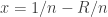
This result actually has a lot of features in common with the optimal result for vaccination. For one thing, it implies that you should always vaccinate if $x > 1/n$ , which is the same lesson that has been repeated above: always vaccinate if there is any chance of an outbreak.

More pointedly, however, you should also always vaccinate any time the relative risk of the disease, $R$ , is larger than 1.

In this sense the self-interested behavior is pretty closely aligned with the globally optimal behavior. The disagreement between them is a relatively mild quantitative one, and exists only when the relative disease risk $R < 1$ .

Confident self-interested behavior

Now, it’s possible that you don’t accept one of the central premises of the analysis in the preceding section. I assumed above that an essentially healthy population is subject to occasional, randomly-occurring moments of “initial exposure”. In such moments it was assumed that a person is chosen at random to be exposed to the disease. Presumably this exposure has to do with either traveling to a foreign location where the disease is endemic, or with meeting someone who has just come from such a location.

You might think, however, that it is very unlikely that your child will ever be such a “primary exposure point”. Perhaps you know that your child is very unlikely to travel to any place where the disease is endemic, or to meet anyone who has come directly from such a place. If you have this kind of confidence, then the calculation changes a bit. Essentially, one needs to remove the probability of being the initial exposure point from the analysis above.

Under these assumptions, the resulting risk of contracting the disease becomes $E T x n/[N(1-xn)]$ , which is smaller than the one listed above by a factor $x n$ . Consequently, the Nash equilibrium shifts to a higher rate of non-vaccination, given by

$x = 1/[n(1+R)]$ . (3)

This equation satisfies the same “no epidemics” rule, but it is qualitatively different in the way it responds to increased disease risk $R$ . Namely, there is never a point where the population achieves complete vaccination.

In other words, a population of “confident” self-interested individuals will always have some finite fraction $x$ of vaccination holdouts, no matter how high the disease risk or how low the vaccine risk. If enough of their fellow citizens are vaccinated, these individuals will consider that the herd immunity is enough to keep them safe.

The three possible non-vaccination rates can be illustrated like this:

vaccination_graph

Real data: the MMR vaccine

The above discussion was completely theoretical: it outlined the ideal rate of vaccination according to a range of hypothetical decision-making criteria. Now let’s look at where the present-day USA falls among these hypotheticals. As a case-study, I’ll look at one of the more hotly-discussed vaccines: the measles-mumps-rubella (MMR) vaccine.

First of all, it is sadly necessary for me to remind people that there is absolutely no evidence for any link between MMR (or any other vaccine) and autism.

But that’s not to say that there is zero risk inherent in the MMR vaccine. In very rare cases, a vaccination can lead directly to a runaway allergic reaction, which can produce seizures, deafness, permanent brain damage, or other long-term effects. The CDC estimates these side effects to occur in at most one person per million MMR vaccinations. (In terms of the variables above, this means $v = 10^{-6}$ .

Compare this to the combined rate of measles, mumps, and rubella infections in the USA. The average rate of occurrence of these diseases during the past five years has been something like 1200 cases per year. Given that the MMR vaccine coverage in the United States is about 92%, this implies a rate of “initial exposure” of something like $1200/0.08 = 15000$ /year across the entire US. (Most exposures do not lead to infection.)

Of course, most people who contract measles, mumps, or rubella recover without any permanent side effects – they just have to suffer through an unpleasant illness for a few weeks. So to make a fair comparison, I’ll discount the exposure rate by a factor that approximates only the risk of acquiring a permanent disability due to the disease. For example, about 0.3% of measles cases are fatal. For mumps, about 10% of cases lead to meningitis, and something like 20% of those result in permanent disability (such as hearing loss, epilepsy, learning disability, and behavioral problems). Finally, the main danger of rubella is associated with congenital rubella syndrome, a terribly sad condition that affects infants whose mothers contract rubella during the middle trimester of pregnancy.

Even discounting this last one, a low-side estimate is that about 1.7% of people who get measles, mumps, or rubella will suffer some form of permanent disability as a consequence. So I’ll discount the “primary exposure” rate to only $E = 0.017 \times 15000 \approx 260$ /year.

This number should be compared to the rate of vaccine-induced disability, which is something like $4$ instances/year (given that about 4 million people get the MMR vaccine per year, and about one per million gets a permanent disability from it). Comparing these rates gives an estimate for the relative disease risk:

$R \approx 70$ .

Pause for a moment: this is a large number.

It implies that the risk associated with actually contracting measles, mumps, or rubella is at least 70 times larger than the risk from the vaccine.

This is true even with the relatively low incidence of cases in the US, and even with the relatively robust “herd immunity” produced by our 92% vaccine coverage. $R = 70$ is also a low-side estimate – there are a number of other disease-related complications that I haven’t taken into account, and I haven’t made any attempt to account for the unpleasantness of getting a disease that you eventually recover from without permanent disability.

Given this large value of relative risk, we can safely conclude the current non-vaccination rate in the USA, $x \approx 8$ %, is way too high. At such a large value of $R$ , both the altruist and the self-interested person will agree that universal vaccination is the right thing to do.

Even the “confident self-interested” person, who believes that their child has no chance of being a point of primary exposure to the disease, will agree that the current vaccine coverage is too low to justify non-vaccination. Only at $x$ less than $1$ % could such a calculation possibly justify non-vaccination in the present-day USA.

Conclusion

I went through this analysis because I believe that, at a theoretical level, there is room for a conversation about weighing the risks of vaccination against the benefits. It is true that in a relatively healthy population that is herd-immunized against outbreaks, a vaccine’s side effects can be a more real risk than the disease itself. It is also worth understanding that in such situations, the incentives of the altruist (who wants to minimize the risk to the world at large) are not perfectly aligned with the incentives of individual parents (who want to minimize the risk to their own child).

But in the present-day USA, these choices do not appear to be at all difficult, and there are no thorny theoretical issues to worry about. Our vaccines remain safe enough, and the disease risks remain large enough, that any level of rational quantitative thinking, self-interested or altruistic, leads to the same conclusion.

Vaccinate your kids.

(Unless, of course, you know that your child has some pre-existing medical condition that makes vaccination unsafe.)

A blog about the big ideas in physics, plus a few other things

Dawn of the Topological Age?

The “shape” of an electron band

Implications of Topology

Topological bands in three dimensions

What technologies will topological materials enable?

References

What are the odds?

What I did right

I prioritized conceptual understanding over technical skill

I learned how to talk about physics, in addition to learning how to do physics

I worked hard to make good talks

I made friends in physics, and I put a lot of effort into maintaining those friendships

I approached well-known, established people for mentorship and collaboration, and I tried to do good work for those people

When I found people who were smarter than me, I tried to learn from them

I was generous, open, and friendly, and avoided being competitive or proprietary

I made an effort to be creative

I was willing to sacrifice from my personal life and my personal relationships when necessary

What I did wrong

I finished my PhD quickly

I avoided fashionable topics

I didn’t spend enough time reading new papers

I allowed my work to become scattered, rather than focusing on a single field

I insisted too often that people explain things in my terms, rather than learning to understand things in their terms

I didn’t prioritize my career over my wife’s career

Ways in which I was lucky

I was uniformly encouraged

I had undergraduate advisors who cared more about my future than about their own research

I ended up with a PhD advisor who (1) was famous, (2) really cared about teaching me, and (3) worked relentlessly to find me opportunities

I went to the Boulder Summer School and made lots of friends, many (most?) of whom remained in academia

I got a postdoc position with an independent travel budget, and I used it to my full advantage

Someone was kind to me and gave me a postdoc job when I was floundering

I befriended people at MIT who became great scientists

Someone was kind to me and kept me on when I was about to fail out

What to make of it all

How thick is the atmosphere?

The Boltzmann Distribution

Footnote:

A simple example

UPDATE:

Gravitational Force

Drag force

Final Answer: never skydive in the rain

Risk and Reward

The optimal behavior

Rational self-interested behavior

Confident self-interested behavior

Real data: the MMR vaccine

Conclusion

Subscribe

Follow Blog via Email

Recent Posts

Top Posts & Pages

Categories