How thick is the atmosphere? A derivation of the Boltzmann distribution

July 14, 2018

by Brian

Let’s talk about a small question as a way of introducing a big question.

How thick is the atmosphere?

How far does Earth’s atmosphere extend into space? In other words, how high can you go in altitude before you start to have difficulty breathing, or your bag of chips explodes, or you need to wear extra sunscreen to protect your skin from UV damage?

You probably have a good guess for the answer to these questions: it’s something like a few miles of altitude. I personally notice that my skin burns pretty quickly above ~10,000 feet (about 2 miles or 3 km), and breathing is noticeably difficult above 14,000 feet even when I’m standing still.

Of course, technically the atmosphere extends way past 2-3 miles. There are rare air molecules from Earth extending deep into space, becoming ever more sparse as you move away from the planet. But there’s clearly a “typical thickness” $h$ of the atmosphere that is on the order of a few miles. Altitude changes that are much smaller in magnitude aren’t noticeable, and altitude changes that are much larger give you a much thinner atmosphere.

What physical principle determines this few-mile thickness?

At a conceptual level, this is actually a pretty simple problem of balancing kinetic and potential energy. Imagine following the trajectory of a single air molecule (say, an oxygen molecule) for a long time. This molecule moves in a sort of random trajectory, buffeted about by other air molecules, and it rises and falls in altitude. As it does so, it trades some of its kinetic energy for gravitational potential energy when it rises, and then trades that potential back for kinetic energy when it falls. If you average the kinetic and potential energy of the molecule over a long time, you’ll find that they are similar in magnitude, in just the same way that they would be for a ball that bounces up and down over and over again.

There is actually an important and precise statement of this equality, called the virial theorem, which in our case says that

$2 \langle \textrm{K.E.}_z \rangle = \langle \textrm{P.E.} \rangle$

where $\langle \textrm{K.E.}_z \rangle$ is the average ~~potential~~ kinetic energy in the vertical direction and $\langle \textrm{P.E.} \rangle$ is the average potential energy.

The gravitational potential energy of a particle of mass $m$ is just

$\textrm{P.E.} = mgh$

and the typical kinetic energy of the air molecule is related to the temperature, (this is, in fact, the definition of temperature):

$\langle \textrm{K.E.}_z \rangle = \frac{1}{2} k_B T$ ,

where $k_B$ is Boltzmann’s constant and $T$ is the absolute temperature (i.e., measured from absolute zero). On the earth’s surface, $k_B T$ is about 25 milli-electronvolts, or $\approx 4 \times 10^{-21}$ Joules.

Using these equations to solve for $h$ gives $h \sim k_B T /(m g)$ , which is about 5 miles.

Everything makes sense so far, but let’s ask a more interesting question: What is the function that describes how the thickness of the atmosphere decays with altitude? In other words, what is the probability density $p(z)$ for a given air molecule to be at altitude $z$ ?

Pastoral scene, with oxygen molecules

Let’s take a God-like perspective on this question [insert joke here about typical physicist arrogance]. Imagine that you could choose some function $p(z)$ from the space of all possible functions, and in order to make your choice you must first ask the question: which function is best?

“Best” may seem like a completely subjective word, but in physics we often have optimization principles that let us define the “best solution” in a very specific way. In this case, the best solution is the one with the highest entropy. Remember that saying “this state has maximum entropy” literally means “this state is the one with the most possible ways of happening”. So what we are really searching for is the function $p(z)$ that is most probable to appear from a random process.

The entropy of a probability distribution $p(z)$ is

$S = - k_B \int_0^\infty p(z) \ln p(z) dz$ ,

This is a generalization of the Boltzmann entropy formula $S = k_B \ln W$ (which is a sufficiently big deal that Boltzmann had it engraved on his tombstone).

Now, there are two relevant constraints on the function $p(z)$ . First, it must be normalized:

$\int_0^\infty p(z) dz = 1$ .

Otherwise, it wouldn’t be a proper probability distribution.

Second, the distribution must correspond to a finite average energy. In particular, the average potential energy of an air molecule must be $k_B T$ . Since the energy of a molecule with altitude $z$ is $m g z$ , we have the second constraint

$\int_0^\infty (m g z) \times p(z) dz = k_B T$ .

Now, for those of you who read the previous post, this kind of problem should start to look familiar. To recap, we want

a function $p(z)$ that maximizes some quantity $S$
and is subject to two constraints

This is a job for Lagrange multipliers!

To optimize the quantity $S$ using Lagrange multipliers, we start by writing the Lagrange function

$\Lambda = S - \lambda_1 [\int_0^\infty p(z) dz - 1] - \lambda_2 [mg \int_0^\infty z p(z) dz - k_B T]$ .

Here, the two quantities in brackets represent the constraints. Putting in the expression for $S$ and then taking the derivative $\partial \Lambda/\partial p$ and setting it equal to zero gives

$-k_B [\ln p(z) + 1] - \lambda_1 - \lambda_2 m g z = 0$

Since $p$ appears only in a logarithm, rearranging and solving for $p(z)$ gives something like

$p(z) = \textrm{const.} \times e^{-\textrm{const.} \times z}$

Now we can use the two constraint (normalization and having a fixed expectation value of the energy) to solve for the values of the two constants. This procedure gives

$p(z) = \frac{1}{h} e^{-z/h}$ ,

where $h = k_B T /(m g)$ is the same “typical thickness” that we estimated at the beginning.

Maybe this seems like a funny little exercise in calculus to you, but what we just did is actually a big deal. We started with very little knowledge of the system at hand: we didn’t know anything about the composition of Earth’s atmosphere, or how air molecules collide with each other, or any principles of physics at all except for the high-school level formula for gravitational potential energy and the understanding that temperature is a measure of kinetic energy. But that was enough to figure out the precise formula for atmospheric density, just by demanding that such a formula must be the most likely one, in the sense of having the highest entropy.

And, it turns out, our derivation is pretty good. Here’s data from the Naval Research Laboratory:

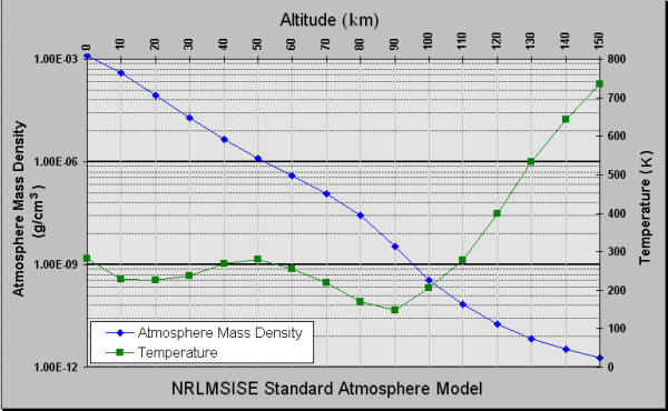
Notice that the density of the atmosphere looks very much like an exponential decay (a straight line on this plot) up until about 80 km of altitude. At higher altitude there’s a sort of crazy increase in temperature (probably due to direct heating from solar radiation and an absence of equilibration with the thicker atmosphere below it) that slows down the decay of atmosphere density.

The Boltzmann Distribution

With a relatively small amount of work, we figured out how thick Earth’s atmosphere is, and how the that thickness depends on altitude.

But it turns out that what we really just did is something much bigger. We found a way to relate energy — in that last problem, expressed through altitude — to probability.

So let’s take a step back, and look over what we did while thinking of a much bigger, more general problem. Suppose that some system (it could be a single particle, or it could be a set of many particles) has many different configurations that it can take. Let’s say, generically, that the energy of some configuration $i$ has energy $E_i$ . Now let’s ask: what is the best probability distribution $p_i$ for describing how likely each configuration is?

Despite knowing literally nothing about the specifics of this problem, we can still approach it in exactly the same way as the last one. We say that the distribution $p_i$ must maximize the entropy:

$S = - \sum_i p_i \ln p_i$ ,

while it is subject to the normalization constraint

$\sum_i p_i = 1$

and the constraint of having a finite average energy $k_B T$ :

$\sum_i E_i p_i = k_B T$ .

These equations all look identical to the ones we wrote down when talking about the atmosphere. So you can more or less just write down the answer now by looking at the previous one, without doing any work:

$p_i = \textrm{const.} \times e^{-E_i/(k_BT)}$ .

Now this formula is a really big deal. It is called the Boltzmann distribution.

The Boltzmann distribution allows you, very generically, to say how likely some outcome is based only on its energy. The only real assumption behind it is that the system has time to evolve in a sort of random way that explores many possibilities, and that its average quantities are not changing in time. (This set of conditions is what defines equilibrium.)

It’s a formula that rears its head over and over in physics, turning seemingly impossible problems into easy ones, where all the details don’t matter. I’m pretty confident that, if I had discovered it, I would put it on my tombstone also.

Footnote:

While I, personally, have used the Boltzmann formula countless times in my life, my favorite application of it was to study pedestrian crowds. It turns out that humans have a very well-defined analogue of “interaction energy” with each other that dictates how they move through crowds. The Boltzmann distribution is what enabled us to figure out how that interaction worked!

13 Comments leave one →

pa32r permalink

July 15, 2018 2:26 pm

Excellent! I’ve done the typical derivation of pressure vs. altitude based on gravity and the mass of the atmospheric column but this is much more satisfying. So far, I’ve only read it through without pencil and paper to follow along but I’ll have my pencil out later today.

Thanks and, again, welcome back!

Reply
- leon rockandroll permalink
  
  July 16, 2018 1:27 pm
  
  would it be possible to look at your derivation? Thanks
  
  Reply
  - PA32R (@PA32R) permalink
    
    July 17, 2018 11:38 pm
    
    Sure, though since I need to do it in my spare time it will be a little while. But, keep in mind, it does not include the variation of temperature with altitude.
    
    Reply
    - @Noel_Carrascal (Leon Rockandroll) permalink
      
      July 20, 2018 2:31 pm
      
      Thanks. That would work. Your derivation and this post will help me start my own inquiry on the subject which I have been too lazy to start on my own. I look forward to it.
Jan permalink

July 17, 2018 8:09 am

Your formula 2 = does not match your description above it;

> it trades some of its kinetic energy for gravitational potential energy when it rises, and then trades that potential back for kinetic energy when it falls.

According to the formula, there would be no trade-off, but proportionality; the higher the molecule gets, the higher the P.E., the higher the K.E. But that is obviously incorrect, at least for molecule acted upon by gravity.

There are various “virial theorems”, but usually none uses ground-based potential energy $mgh$. Instead, potential energy relative to infinity is used: GMm/r. And there is a minus sign; for gravity, 2 = – .

So your derivation of the average height h = k_B T/(mg) is incorrect.

If one uses an assumption that atmosphere has single temperature (rough approximation), it is easier to argue based on the generalized equipartition theorem for Hamiltonian H = 1/2mv^2 + mgh. Then the average potential energy of the molecule mgh is of order k_B T. This immediately implies the average height h=k_B T/(mg).

Reply
- Brian permalink*
  
  July 17, 2018 10:30 am
  
  Hi Jan,
  
  Sorry, you’re right. The equipartition theorem was probably what I should have gone with, instead of the virial theorem.
  
  But for the point of being pedantic, I actually think that what I said isn’t technically wrong. Suppose I have a system of two particles, with the z-dependent interaction energy $V(z) = m g z$ . This is like the interaction between a molecule and the planet earth, at z much shorter than the earth radius.
  
  Then the virial theorem gives $2\langle T \rangle = + \langle V \rangle$ , with a positive sign, and everything is the way I said.
  
  Reply
  - Jan permalink
    
    February 12, 2019 9:05 am
    
    No I take that back, it wasn’t clear to me initially but I agree now the virial theorem can be used the way you did, as the pressure forces from the ground have zero contribution to virial if P.E. is zero on ground. The only problem that I see now is that this equation Av(2K.E.) = Av(P.E.) is about time average of energy of the whole set of molecules in the model 1D atmosphere. But effective temperature of gas is determined by average of kinetic energy _over_molecules_ there, not average of net kinetic energy over time. So some ergodic behaviour has to be assumed as well, which would be worth mentioning in the article. Without it, the virial theorem allows for the whole atmosphere to get very hot, say 6000 K, for arbitrarily long period of time.
    
    Reply
    - Jan permalink
      
      February 12, 2019 9:11 am
      
      Thinking more about it, if at some time we have instantaneous values that obey K.E.=1/2P.E., then the kinetic energy can rise later to value 3x as large, so the temperature would rise from 300K to 900K. So, not as dramatic as I wrote above, but still a good thing that it doesn’t happen.
- Brian permalink*
  
  July 17, 2018 10:41 am
  
  I think the (apparent) disagreement between your formulae and mine is about where you put the reference for potential energy. You are writing V = -G M m/r, which implies zero potential energy infinitely far away, while I am writing V = m g h, which implies zero potential energy at the surface.
  
  Reply
Jan permalink

July 17, 2018 8:12 am

The site removed some formulae from my post, probably because they contained characters “lower than” and “higher than”. Here’s what I meant:

… Your formula 2K.E._z = P.E.

… And there is a minus sign; for gravity, 2K.E. = – P.E.

Reply
RichardLH permalink

July 19, 2018 1:34 pm

So what is the density/gravity function for a completely gaseous body? All the way through. We know, from Newton, that at the centre of any body the gravitational field returns to a local 0, i.e. there is equal amounts of mass ‘above and ‘below’. So what is for a gas? Or, for than matter (pun) a disc shaped galaxy which can also be considered to be a very diffuse gas of sorts as well.

Reply
Lagrangian Mechanic permalink

August 1, 2018 12:15 am

One of my favorite lectures in 8.044 (statistical mechanics) many many years ago was the one where the professor started with the microcanonical ensemble and over the course of the 90 minute lecture derived the Maxwell-Boltzmann distribution.

Reply