Entropy and gambling

Entropy is one of those terms that everyone learns in high school and no one really understands.  That’s because it usually gets defined in extremely vague terms, like “entropy is the amount of disorder in a system.”  Well, what do you mean by disorder?  How can something defined so loosely be used in precise equations?  And what, exactly, does it mean to say “a system tends to settle into a state of maximum entropy”?  With this post I’ll try to demystify entropy a little bit by talking about a simple gambling game, where betting on the “outcome with highest entropy” proves to be a successful strategy.

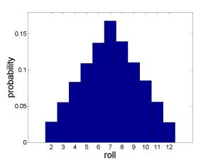
Consider the simplest possible gambling game: you roll some dice and try to guess the outcome.  With a single die, there is nothing interesting to talk about.  Every possible value 1 – 6 is equally likely (probability 1/6).  But what about with two dice?  It turns out that not all outcomes are equally probable.  After all, there are six ways of rolling a 7 — 1 then 6 (which I’ll denote {1 ,6}) or {2,5} or {3,4} or {4,3} or {5,2} or {6,1} — but only one way of rolling a 12:{6, 6}.  So if you’re going to bet on an outcome, picking 7 is a much better idea than picking 12 (six times better!  remember this for future gambling purposes).  If you wanted to plot the probabilities of each roll, it would look like this:

Rolling 2 dice

Since 7  is the most likely roll, and we know that “a system settles into its state of maximum entropy”, it must be true that 7 is the outcome with the highest entropy.

Here I should mention that while we think of entropy in vague “disorder” terms, it actually does have a very precise definition.  Entropy S can be defined through the Boltzmann definition:

where is the number of possible configurations that lead to a particular outcome ( is just a constant that gives the entropy convenient units).  Since there are six distinct ways of rolling a 7, the entropy of a roll of 7 is .

So 7 is the roll with the highest entropy.  But entropy doesn’t seem like a terribly useful definition here.  The system is supposed to “settle into the state with the highest entropy”, but it’s not like you’re going to roll a 7 every time you play.  So what gives?

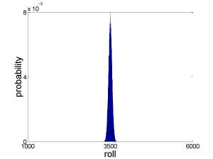
The answer is that the idea of entropy was never meant to be useful for a system of only two things (here, two dice).  It is a “thermodynamic quantity”, meaning it is useful in describing systems of many, many separate things.  So let’s extend our gambling game to a larger scale.  Suppose now that you’re betting on the outcome of rolling 1,000 dice.  What number should you bet on?  Here is the outcome of 100,000 computer-simulated dice rollings:

Rolling 1000 dice

This result is a little surprising.  We could theoretically roll anything between 1,000 (all 1’s) and 6,000 (all 6’s).  But apparently rolling a number close to 3,500 is overwhelming more likely than any other.  That’s because there are many, many more ways of rolling a 3500 than of rolling any number close to 1000 or 6000 (just to put a number to it, there are about distinct ways of rolling a 3500).  3500 is the “state of maximum entropy”, and it is clear that with 1000 dice our system is “settling into” that state.   It is no coincidence that the most likely roll is equal to 3.5 times the number of dice, since 3.5 is the average roll for a single die (the average of 1, 2, 3, 4, 5, and 6).  If you were to play this game with even more dice, you would find that the probability distribution becomes increasingly sharp, centered around 3.5 times the number of dice.

Real thermodynamics, the study of the bulk behavior of large collections of things, is like a game played with dice.  You can imagine what a probability distribution would look like if we rolled that many dice — you would be a fool to bet on any outcome that differed from by more than a millionth of a percent!  Or, put another way, the average roll per die will be extremely close to 3.5.  That’s why, when we describe a system with random objects, like a fluid composed of individual molecules, the overall energy or pressure or momentum is easy to predict.  Because even though individual components may fluctuate very widely, there are some totals (like the sum of the dice) that are much more likely than others.  These are the states of maximum entropy.

So, in the end, it sounds a bit silly to say that “a system tends to settle into a state of maximum entropy”.  It’s a bit like saying “a system tends to be in the state it is most likely to be in”.  Nonetheless, talking about increasing entropy can still be a useful idea.  For one thing, we have seen that the “most likely states” tend to be overwhelmingly likely, so that the “maximum entropy state” is not just probable, but virtually certain.  There’s also nothing wrong with associating entropy with “disorder”.  In a game of 4 dice, for example, a roll like {3,2,5,4} or {1,5,6,2} (both of which give 3.5 * 4 = 14, the state of maximum entropy) looks more “disorganized” than a roll like {1,1,1,1} or {6,6,5,6}.  Even though all four of those individual sequences are equally likely to occur, the more “disorganized – looking” ones tend to belong to likely totals, while the the “organized – looking” ones tend to belong to unlikely totals.  This is the main idea behind entropy.