Guest Post: If You Walk in A Closed Loop, Do You End Up Where You Started?

Editor’s note: The following is a guest post contributed by Anshul Kogar.  Anshul is a postdoctoral researcher in experimental condensed matter physics who currently splits his time between Argonne National Laboratory and the University of Illinois at Urbana-Champaign.  He maintains the blog This Condensed Life, which discusses conceptual ideas and recent developments in condensed matter physics.

 

This may surprise you, but the answer to the question in the title leads to some profound quantum mechanical phenomena that fall under the umbrella of the Berry or geometric phase, the topic I’ll be addressing here. There are also classical manifestations of the same kind of effects, a prime example being the Foucault pendulum.

Let’s now return to the original question. Ultimately, whether or not one returns to oneself after walking in a closed loop depends on what you are and where you’re walking, as I’ll describe below. The geometric phase is easier to visualize classically, so let me start there. Let’s consider a boy, Raj, who is pictured below:

Raj

Now, Raj, for whatever reason, wants to walk in a rectangle (a closed loop). But he has one very strict constraint: he can’t turn/twist his body while he’s walking. So if Raj starts his walk in the top right corner of the rectangle (pictured below) and then walks forward normally, he has to start side-stepping when he reaches the bottom right corner to walk to the left. Similarly, on the left side of the rectangle, he is constrained to walk backwards, and on the top side of the rectangle, he must side-step to the right. The arrow in the diagram below is supposed to indicate the direction which Raj faces as he walks. When Raj returns to the top right corner, he ends up exactly in the same place that he did when he started — not very profound at all! But now let’s consider the case where Raj is not walking on a plane, but walking on the surface of a sphere:

Again, the arrow is supposed to indicate the direction that Raj is facing. This time, Raj starts his trek at the north pole, heads to Quito, Ecuador on the equator, then continues his walk along the equator and heads back up to the north pole. Notice that on this journey, even though Raj obeys the non-twisting constraint, he ends up facing a different direction when he returns to the north pole! Even though he has returned to the same position, something is slightly different. We call this difference anholonomy.

Why did anholonomy result in the spherical case and not the flat rectangle case? Amazingly, it turns out to be related to the hairy ball theorem (don’t ask me how it got its name). Crudely speaking, the hairy ball theorem states that if you have a ball covered with hairs, you can’t comb the hairs straight without leaving at least one little bald spot or tuft. In the image below you can see a little tuft on both the top and bottom of the sphere:

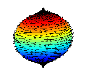The sphere which Raj traversed had a little bald spot at the north pole, leading to the anoholonomy.

Now before moving onto the Foucault pendulum, I want to explicitly state the items that were critical in obtaining the anholonomy for the spherical case: (i) The object that is transported must have a direction (i.e. be a vector); (ii) The object must be a transported on a surface on which one cannot properly comb hair.

Now, how does the Foucault pendulum get tied up in all this? Well, the Foucault pendulum, swinging in Paris, does not oscillate in the same plane after the earth makes a full 24-hour rotation. This difference in angle between the original and the next-day plane of oscillation is also an anholonomy, except the earth rotates instead of the pendulum taking a walk. Check out this great animation from Wikipedia below:

If the pendulum was at the north (south) pole, the pendulum would come back to itself after a 24-hour rotation of the earth, (). If the pendulum was at the equator, the pendulum would not change its oscillation plane at all (). Now, depending on the latitude in the northern hemisphere where a Foucault pendulum is set up, the pendulum will make an angle between and after the earth makes its daily rotation. The north pole case, in light of the animation above, can be inferred from this image by imagining the earth rotating about its vertical axis:

The concept on anholonomy in the quantum mechanical case can actually be pictured quite similarly to the classical case described above. In quantum mechanics, we describe particles using a wavefunction, which in a very basic sense is also a vector. The vector does not exist in “real space” but what physicists refer to as “Hilbert space”. Nonetheless, the geometrical game I played with classical anholonomy can also be played in this abstract “Hilbert space”. The main difference is that the anholonomy angle becomes a phase factor in the quantum realm. The correspondence is as so:

(Classical)         (Quantum)

The expression on the right is precisely the Berry/geometric phase.  In the quantum case, regarding the two criteria above, we already have (i) a “vector” in the form of the wavefunction — so all we need is (ii) an appropriate surface on which hair cannot be combed straight. It turns out that in quantum mechanics, there are many ways to do this, but the most famous is undoubtedly the case of the Aharonov-Bohm effect.

In the Aharonov-Bohm experiment, one prepares a beam of electrons, splits the beam and passes them on either side of the solenoid, recombining them on the other side. A schematic of this experimental steup is shown below:

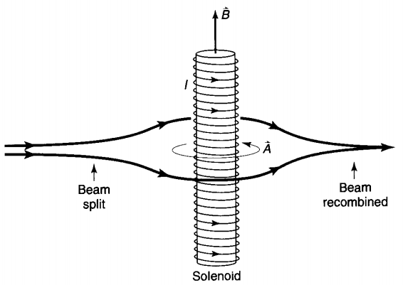
In the image, B labels the magnetic field and A is the vector potential. While many readers are probably familiar with the magnetic field, the vector potential may not be as household a concept. The vector potential was originally thought up by Maxwell, and considered to be a mathematical oddity. He realized that one could obtain B by measuring the curl of A at each point in space, but A was not given any physical meaning.

Now, it doesn’t immediately seem like this experiment would give one a geometric phase, especially considering the fact that the magnetic field outside the solenoid is zero. But let’s take look at the pattern for the vector potential outside the solenoid (top-down view):

Interestingly, the vector potential outside the solenoid looks like it would have a tuft in the center! Criterion number (ii) may therefore potentially be met. The one question left to be answered is this: can the vector potential actually “rotate” the electron wavefunction (or “vector”)? The answer to that question deserves a post to itself, and perhaps Brian or I can fill that hole in the future, but the answer seems to be emphatically in the affirmative.

The equation describing the relationship between the anholonomy angle and the vector potential is:

where is the rotation (or anholonomy) angle, the integral is over the closed loop of the electron path, and is just a proportionality constant.

The way to think about the equality is as so: is an infinitesimal “step” that the electron takes, much in the way that Raj took steps earlier. At each step the wavefunction is rotated a little compared to the previous step by an amount , dictated by the vector potential. When I add up all the little rotations caused by  over the entire path of the electrons, I get the integral around the closed loop.

Now that we have the anholonomy angle, we need to use the classical quantum relation from above. This gives us a phase difference of between the electrons that go to the right and left of the solenoid. Whenever there is a non-zero phase difference, one should always be able to measure it using an interference experiment — and this is indeed the case here.

An experiment consisting of an electron beam fired at double-slit interference setup coupled with a solenoid demonstrates this interference effect most profoundly. On the setup to the left, the usual interference pattern is set up due to the path length difference of the electrons. On the setup to the right, the entire spectrum is shifted because the extra phase factor from the anholonomy angle.

Again, let me emphasize that there is no magnetic field in the region in where the electrons travel. This effect is due purely to the geometric effect of the anholonomy angle, a.k.a. the Berry phase, and the geometric effect arises in relation to the swirly tuft of hair!

So next time you’re taking a long walk, think about how much the earth has rotated while you’ve been walking and whether you really end up where you started — chances are that something’s just a little bit different.