Spare me the math: the Lamb Shift

April 24, 2013

by Brian

To kick off SMTM, I’ll look at a topic that I never really understood when I was in graduate school: the Lamb shift.

The Lamb Shift: what it is

In its most commonly-discussed form, the Lamb shift is a small effect. In fact, it’s a very small effect (which is probably why I never bothered to learn it in the first place). The Lamb shift is a miniscule change in (some of) the energy levels of the hydrogen atom relative to where it seems like they should be. For example, the binding energy of an electron to the hydrogen nucleus (a proton) is about $13.6$ electron volts. The Lamb shift is a phenomenon that changes this energy level by about $4\times10^{-6}$ eV, or about $0.00003$ %. But the existence of this shift was a serious puzzle to physicists in the 1940s and 50s, and its final resolution provided a beautiful piece of physics that helped spur the development of quantum electrodynamics, one of the most spectacularly successful scientific theories in history.

The essence of the Lamb shift can be stated like this: it is the energy of interaction between hydrogen and empty space.

The dominant contribution, of course, to the energy of the hydrogen atom is the interaction of the electron with the proton it’s orbiting. If you want a really quick way to derive the energy of the hydrogen atom, all you need to remember is that the size of the electron cloud around the proton has some characteristic size $a$ . Confining the electron to within this cloud costs some kinetic energy $\sim \hbar^2 /m a^2$ , and it buys you some energy of attraction, $\sim -e^2/a$ (here I’m being too lazy to write out the $4\pi\epsilon_0$ s that come in SI units). So the total energy is something like $E \sim \hbar^2/ma^2 - e^2/a$ . If you minimize $E$ with respect to $a$ (take the derivative and set it to zero), you’ll find that

$a \sim \hbar^2/me^2$

and

$E \sim -me^4/\hbar^2 \sim -e^2/a$ .

The constant $a \approx 0.5$ Angstroms is the Bohr radius, which is the typical size of the hydrogen atom (and, roughly speaking, any atom). The energy $-e^2/a \equiv R$ is the Rydberg energy.

The Lamb shift comes from the way this balanced state between electron and proton is influenced by the slight, random buffetings from the vacuum itself.

$\hspace{1mm}$

The hydrogen atom

There are two players in this story: the hydrogen atom, and empty space. I’ll describe the former first, since the latter (paradoxically) is considerably harder.

In reality, the Lamb shift is most easily observed in excited states of hydrogen (the P states, see Footnote 1 at the bottom), but for the purpose of this discussion it’s easiest to think about the ground state. In terms of the electron probability cloud, the ground state of the hydrogenic electron looks like this:

It has a peak right at the middle of the atom, and it falls of exponentially.

I know there is a lot of trickiness associated with whether to think about an electron as a particle or as a wave (my own favorite take is here — in short, an electron is a particle that surfs on a wave), but for this discussion it’s easiest to think of an electron as a point object that just happens to arrange itself in space according to the probability density plotted above.

$\hspace{1mm}$

The vacuum

There is a lot going on in empty space. If this crazy idea is completely new to you, I would (humbly) suggest reading my post on the Casimir effect. The upshot of it is that all of space is filled by endlessly boiling quantum fields, and one of these, the electromagnetic field, is responsible for conveying electromagnetic forces. As a result of its indelible boiling, however, the electromagnetic field can push on charged objects, like our electron, even when there are no other charged objects around to seemingly initiate the pushing.

To get a better description of the electromagnetic field in vacuum, it will be helpful to imagine that our electron sits inside a large metal box with size $L$ . Inside this metal box are lots of randomly-arising electromagnetic waves (“virtual photons”). Something like this:

When dealing with quantum fields, a good rule of thumb is to expect that, in vacuum, every possible oscillatory mode will be occupied by one quantum of energy. In this case, it means that for every possible vector $k = 2\pi / \lambda$ , where $\lambda = 2L, 2L/2, 2L/3, 2L/4, ...$ is a permissible photon wavelength, there will be roughly one photon present inside the box. This photon has an energy $E_k = \hbar c k$ , where $c$ is the speed of light. One can estimate the typical magnitude of the electric field the photon creates, $|\vec{\mathcal{E}_k}|$ , by remembering that $|\vec{\mathcal{E}_k}|^2$ gives the energy density of an electric field. Since the photon fills the whole box, this means that $|\vec{\mathcal{E}_k}|^2 \times L^3 \sim E_k$ , or $|\mathcal{E}_k|^2 \sim \hbar c k/L^3$ . This electric field oscillates with a frequency $ck$ .

So now the stage is set. The hydrogen atom sits inside a “large box” (which we’ll do away with later), and inside the box with is a huge mess of random electric fields that can push on the electron. Now we should figure out how all this pushing affects the hydrogen energy.

[By the way, you may be bothered by the fact that all these randomly-arising photons seem to endow the interior of the box with an infinite amount of energy. If that is the case, then there’s nothing much I can say except that you and I are in the same club, with only speculation to assuage our uneasiness.]

$\hspace{1mm}$

How the vacuum pushes on hydrogen

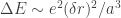
The essence of the Lamb shift is that the random electric fields push on the electron, and in doing so they move it slightly further away from the proton, on average, than it would otherwise be. Another way to say this is that the distribution of the electron’s position gets blurred over some particular (small) length scale $\delta r$ . In particular, the sharp peak in the distribution near the center of the atom should get slightly rounded, like this:

The “smearing length” δr is greatly exaggerated in this picture.

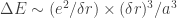
The resulting shift of the electron distribution away from the center lowers the interaction energy of the electron to the proton. To estimate the amount of energy that the electron loses, you can think that in those moments where the electron happens to approach be within a distance $\delta r$ of the nucleus, it frequently finds itself getting pushed outward by an amount $\delta r$ . As a result of this outward push it loses an energy $e^2/\delta r$ . This means that the Lamb shift energy

$\Delta E \sim (e^2/\delta r) \times [\text{fraction of time the electron spends within } \delta r \text{ of the nucleus}]$

$\Delta E \sim (e^2/\delta r) \times (\delta r)^3/a^3$

$\Delta E \sim e^2 (\delta r)^2/a^3$

Now all that’s left is to estimate $\delta r$ .

$\hspace{1mm}$

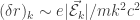
The trick here is to realize that all of those photons within the metal “box” are independently shaking the electron, and each push is in a random direction. So if some photon with wave vector $k_1$ produces, by itself, a displacement of the electron $(\delta r)_{k_1}$ , then the total displacement $(\delta r)$ satisfies

$(\delta r)^2 = (\delta r)^2_{k_1} + (\delta r)^2_{k_2} + (\delta r)^2_{k_3} ...$

[This is a general rule of statistics: independently-contributing things add together in quadrature.]

A photon is essentially just an electric field that keeps reversing sign.

In our case, each $(\delta r)_k$ comes from the influence of a photon, which has electric field $\vec{\mathcal{E}_k}$ . The simplest way to estimate $(\delta r)_k$ is to imagine that the electric field $\vec{\mathcal{E}_k}$ pushes on the electron for a time $\tau \sim 1/kc$ (the period of its oscillation), after which it reverses its direction (as shown on the right). During that time, the acceleration of the electron is something like $|\vec{A}| \sim |\vec{F}|/m$ , where $\vec{F} = e\vec{\mathcal{E}_k}$ is the force of the electric field pushing on the electron, and its net displacement $(\delta r)_k \sim |\vec{A}| \tau^2$ . This means

$(\delta r)_k \sim e |\vec{\mathcal{E}_k}|/mk^2 c^2$ .

$\hspace{1mm}$

Now we should just add up all the $(\delta r)^2_k$ s. Since there is a very large number of photons with a nearly continuous range of energies (due to the very large size of the confining “box”), we can replace a sum over all $k$ ‘s with an integral: $\sum_k (\delta r)^2_k\rightarrow L^3 \int d^3 k (\delta r)^2_k$ . Inserting the expressions for $(\delta r)_k$ and $|\vec{\mathcal{E}_k}|^2$ gives the following:

$(\delta r)^2 \sim (e^2 \hbar/m^2 c^3) \int (1/k) dk$ .

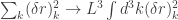
You can notice that the size $L$ of the box drops out of the expression, which is good because the box was completely fictitious anyway.

The only remaining thing to figure out is what to do with the integral $\int(1/k) dk$ , which is technically equal to infinity. In physics, however, when you get an infinite answer, it means that you forgot to stop counting things that shouldn’t actually count. In this case, we should stop counting photons whose wavelength is either too short or too long to affect the electron. On the long wavelength side, we should stop counting photons when their wavelength gets bigger than the size of the atom, $a$ . Such long wavelength photons make an electric field that oscillates so slowly that by the time it has changed sign, the electron has likely moved to a completely different part of the atom, and the net effect is zero. One the short wavelength side, we should stop counting photons when their wavelength gets shorter than the Compton wavelength. Such photons are super-energetic, with energy larger than $mc^2$ , which means their energy is so high that they don’t push around electrons anymore: they spontaneously create new electrons from the vacuum. [In essence, it doesn’t make sense to talk about electron position at length scales shorter than the Compton wavelength.]

Using these two wavelengths as the upper and lower cutoffs of the integral gives $\int (1/k) dk = ln(1/\alpha)$ . Here, $\alpha = e^2/\hbar c \approx 1/137$ is the much-celebrated fine structure constant.

[It is perhaps worth pausing to note, as so many before me have done, what a strange and interesting object the fine structure constant is. $\alpha$ contains only the most fundamental constants of electricity, quantum mechanics, and relativity, ( $e, \hbar$ , and $c$ ), and they combine to produce exactly one dimensionless number. How strange that this number should be as large as 137. As a general rule, fundamental numbers produced by the universe are usually close to $1$ .]

$\hspace{1mm}$

Now we have all the pieces necessary to assemble a result for the Lamb shift. And actually, if you like the fine structure constant, then you’ll love the final answer. It looks like this:

$\Delta E/R \sim \alpha^3 \ln(1/\alpha)$ .

$\hspace{1mm}$

At the beginning of this post I mentioned that the Lamb shift is very small — only about 1/500,000 of the energy of hydrogen (the Rydberg energy, $R$ ). Now, if you want to know why the Lamb shift is so small, the best answer I have is that the Lamb shift is proportional to $\alpha^3$ , and in our universe the fine structure constant $\alpha$ just happens to be a small number.

It’s interesting to note that if we somehow lived in a universe where $\alpha$ was not so small, then the Lamb shift would get big, and those random fluctuations of the quantum field would get large enough to completely knock the electron off the nucleus. This would be a universe without atoms, and consequently, without you and me.

$\hspace{1mm}$

Footnotes

Probability clouds for different hydrogen states. Different states along the same row are supposed to have the same energy, but the Lamb shift splits the S states from the P and D states.

1) You might notice that the Lamb shift appeared only because the electron probability cloud had a peak at the center of the atom. If it didn’t have a peak — say, if it went to zero near the center — then there would be no Lamb shift. This is in fact exactly how the Lamb shift was discovered. Certain excited states of the hydrogen atom have a peak near the center and others go to zero. So while normal quantum mechanics predicts that, say, the 2S and 2P states (shown to the right) have the same energy, in fact the Lamb shift makes a small difference between them. This difference can be observed as a faint ~~radio wave~~ microwave signal from interstellar hydrogen.

2) It’s probably worth noting that if you increased the fine structure constant $\alpha$ , you would have run into bigger problems long before you started fussing about the Lamb shift.

3) Also, while $\alpha$ is a small number in our normal world, it’s not hard to imagine synthetic worlds (the interior of certain materials) where $\alpha$ is not a small number. For example, graphene is a material inside of which there is an effective speed of light that is 300 times smaller than $c$ . This makes $\alpha$ very close to 1, and the sort of effects discussed in this post get very real. This is part of why there has been so much ado about graphene among physicists: it’s quite an exciting (and frustrating) playground for people like me.

UPDATE:

4) I just came across this video of Freeman Dyson (one of my personal favorite physicists) explaining the Lamb shift and some of the history behind it. His conceptual summary of it starts at 2:43.

FURTHER UPDATE:

5) A reader points out to me that the lovely qualitative argument presented here was first put forward by American physicist Ted Welton, in 1948.

Sadly, Welton doesn’t have a Wikipedia article in English (although he does in German). Would anyone like to create one for him?

27 Comments leave one →

brengleman permalink

April 25, 2013 4:27 am

I really enjoyed your post. There was a lot that I missed, but a lot that I took in. I would suggest for people that don’t have the physics experience that you have, to define every variable. You don’t necessarily have to explain every single one, but it would be nice what every variable stood for in your equations.

Thanks again. Good post, and good blog.

Reply
- Brian permalink*
  
  April 25, 2013 8:24 am
  
  Sorry. I hate when people do that. I think what I missed is that $\hbar$ is Planck’s constant (divided by $2\pi$ ), $m$ is the electron mass, and $e$ is the electron charge.
  
  Reply
Steve? permalink

April 25, 2013 4:41 pm

Why does the Lamb shift only matter at the center of the electron distribution? I reread that section a few times and it seems like the electron should be equally buffeted in all space.

Reply
- Brian permalink*
  
  April 25, 2013 5:02 pm
  
  Hi Steve,
  
  You’re right; the electron does get equally buffeted in all space. But for most of the time, that small buffeting (which displaces the electron by about 0.1 femtometers) doesn’t really matter. After all, who cares whether the electron is 1 angstrom away from the nucleus, or 1.000001 angstroms away. If the electron happens to be very close the nucleus, on the other hand, that very small displacement makes a big difference in the attraction energy between the electron and the proton.
  
  Reply
NN permalink

September 29, 2014 5:48 pm

Good explanation.
Quick follow-up question: does the Lamb shift also broaden the lines affected by it? (Which would be my instinctive expectation)

Reply
- Brian permalink*
  
  September 29, 2014 5:59 pm
  
  At the moment I don’t see a reason why the Lamb shift should produce line broadening. What did you have in mind?
  
  Reply
NN permalink

September 30, 2014 9:25 am

If the Lamb shift is caused by “buffeting” of the electron by random fluctuations of the vacuum EM field (which seem to presumably have a noise-like associated spectrum in phase and temporal intensity) then of course this would indeed only “smear out” the centralized maxima of the s-orbital wavefunction on average. But it also seems that such buffeting it would have a time-fluctuating component to the way that it “smeared out” orbital function ( a little like doppler broadening or brownian motion in a centralized potential trap) so that the line would not only be shifted to slightly lower energy but also broadened. (Though the shift is so small that such broadening might very well be immeasurable).

Or have I missed something?

Reply
- Brian permalink*
  
  October 1, 2014 9:33 am
  
  Hi NN,
  
  The way I think about spectral broadening is that it comes from averaging over a bunch of different atoms, each one of which is in a slightly different environment. For example, if you have random stray electric fields, then each hydrogen atom sits in a different electric field, which shifts the electron energy levels by a bit (the Stark effect). This means that the observed absorption frequencies are pulled from a statistical distribution rather than all having one specific value.
  
  The Lamb shift, on the other hand, corresponds to a set of quantum fluctuations that every atom feels in the same way. So there is no reason to think that it produces a “distribution of energies” between different atoms. The electron just has to arrange its wavefunction in a way that accounts for the quantum fluctuation.
  
  Perhaps another way to say this is that the relevant quantum fluctuations are extremely fast with respect to the characteristic orbital period of the electron. I didn’t mention it above, but the scale of the “smearing” of the electron wavefunction is $\delta r \approx 10^{-13}$ meters. At such small length scales the relevant vacuum fluctuations have frequency $c/(\delta r) \approx 10^{21}$ Hz, as compared to the typical atomic orbital frequency $\approx 10^{16}$ Hz.
  
  What this means is that when you attempt to excite an electron from its atomic orbital by shining “slow” light of frequency $\approx 10^{16}$ Hz, you are only seeing the average behavior of the quantum field. So you can’t think that different atoms will see the field differently, and look like they are in “different environments”.
  
  …Of course, I guess this all means that the short answer to your question is “yes, the broadening is so small that it is immeasurable.” 🙂
  
  Reply
Mark Decker permalink

October 5, 2014 9:58 am

I am confused on the explanations for QED’s infinity and the getting rid of it. I watched the Dyson video and a few others on that site. There is discussion of mass renormalization, also the concept of infinite self field strength because the electron is a point with no real radius and finally – your explanation in terms of cutting off the high and low wavelengths and being left with a finite parameter that will affect the electron. Do all of these apparently different concepts relate somehow? If so, how? Thanks.

Reply
- Brian permalink*
  
  October 5, 2014 12:42 pm
  
  Hi Mark,
  
  Probably the most intelligent thing I can say about all those things is that infinities tend to pop up a lot in quantum field theory. The basic reason, as I see it, is that any quantum field apparently has one quantum of energy for every possible wavelength. So, for example, the “box of photons” that I drew above has energy $h c /\lambda$ for every possible wavelength $\lambda$ . But there is apparently no limit to how small $\lambda$ can be, since you can keep subdividing free space as much as you want, so you can arrive at the result that this apparently empty metal box actually has infinite energy inside it.
  
  The common way to resolve this problem is to imagine that eventually, at small enough wavelengths, there won’t be quantum oscillations anymore, so the energy of the field doesn’t actually go to infinity. (This “smallest wavelength” is commonly imagined to be the Planck length, about $10^{-35}$ m.) This is something like imagining that eventually, if we could look close enough at free space, we would find that it wasn’t continuous anymore, but was made out of discrete points with a particular spacing. As it turns out, though, it doesn’t matter for most theories how small this “ultimate spacing” is, as long as it’s very small. So there are places where the energy of something you calculate goes to infinity, and you just say “ahh, but it’s probably not really infinity. And as long as I the divergence of energy gets cut off somewhere I can get a respectable answer.”
  
  Reply
Devin permalink

November 20, 2014 2:38 pm

Excellent post!

However, I’m a little confused about your aside regarding infinite energy in a quantum box. Why would you assume that random fluctuations of an infinite number of states translates to infinite energy? I’ll describe the way I think about it and you can tell me if I’m confused.

In this theoretical framework, it’s the field that’s perturbed, not an observable like energy. Since we have many completely random fluctuations of a field, it’s natural to assume that all those random fluctuations average out to nothing when you consider any one observable.

As an example, sine waves on a string carry energy like the square of the amplitude of the waves. However, if you were to randomly put every possible sine wave on an infinite string at the same time, the string would always appear flat and the energy density would appear to be zero.

When you modify the vacuum electric field by, say, inserting a proton somewhere, the vacuum field fluctuations are no longer completely random because they can see a charge distribution. If you then probe the resulting field by moving an electron around, you should see a difference between a system with infinite not-quite-random field fluctuations and a system with no fluctuations at all. This is the difference between considering an atom in a quantum field (which results in the Lamb shift) and an atom in a classical field (which doesn’t lead to the Lamb shift).

Am I missing something?

Reply
- Brian permalink*
  
  November 22, 2014 10:52 am
  
  Hi Devin,
  
  Thanks, I’m glad you liked the post!
  
  I think what you’re saying is that if you have a huge number of randomly-out-of-phase electric fields (or oscillatory modes on a string), then their amplitude should average out to zero and you’ll essentially have no energy in the box (or very little), rather than an infinite amount.
  
  I think my disagreement with this statement is essentially a statistical one. It’s true that the average value of the electric field must be zero, since positive and negative values of the electric field are equally probably. But that doesn’t mean that the typical magnitude of the electric field at any given point in space is very small.
  
  To see this is in a simple way, try randomly choosing either -1 or +1 a very large number of times and then adding up all the +/-1’s. The answer you get is equally likely to positive or negative, but in a typical realization of this process its value will be actually fairly large. For example, if you add a million +/- 1’s, the sum will be something like 1000 rather than something close to zero. More generally, if you add $N$ random +/- 1’s, the answer you get will be as large as $\sqrt{N}$ , with a random sign.
  
  So, if I say that a metal box has an infinite number of random electric fields in, that means that the magnitude of the electric field at any given point will also go to infinity (with a random sign). This implies an infinite amount of energy inside the box, which seems a little discomforting, philosophically.
  
  Reply
  - Devin permalink
    
    November 22, 2014 2:15 pm
    
    Brian,
    
    In light of your comment, what I said before was too vague. I agree with your statement about the statistics of random values but I thought the situation you just described is different than the situation for a quantum field.
    
    I think what is meant by “every possible oscillatory mode will be occupied by one quantum of energy” in your original post is that we have a complete set of quantum states and when we take an expectation value we’re equally likely to observe any one of them. For the simplest possible quantum in a box this raises the issue of infinite energy because in practice you’d always observe some high energy state. But this is different for a field in vacuum isn’t it? If we take an expectation value of energy over a given region shouldn’t the number of states of the system dictate that energy density in the region of observation is very small?
    
    Devin
    
    Reply
  - Brian permalink*
    
    December 8, 2014 1:06 am
    
    Hi Devin,
    
    Despite my very slow reply, I’m still not sure that I’m properly interpreting your question. But maybe I can rephrase the vacuum energy question this way:
    
    In quantum field theory, one essentially imagines that at every spatial point there is a little harmonic oscillator, and that these harmonic oscillators are connected to each other (this is like the “fabric of tiny springs” picture I was espousing in an earlier post). Each of these harmonic oscillators has one quantum of energy. Since there are (presumably) an infinite number of points in space, the quantum field has an infinite amount of energy in any finite volume.
    
    This picture of every possible point in space having one quantum of energy is equivalent to having one quantum of energy for every possible mode — or one photon per possible wavelength.
    
    Reply
    - shortda permalink
      
      December 12, 2014 7:10 pm
      
      Brian,
      
      Thanks for your reply. That certainly sounds paradoxical given my knowledge about quantum oscillators but I always assumed that the field theory was more subtle. I think I don’t have enough command of the QFT formalism to get my head around the field version yet. Do photons have creation and annihilation operators like other particles? If so, how would you write down the quantum field in vacuum? Do you actually have to add up photon creation operations at each point in space?
      
      Devin
    - Brian permalink*
      
      December 12, 2014 8:16 pm
      
      Hi Devin,
      
      Now you’re asking really tricky questions. The short answer: yes, there are creation/annihilation operators for photons, just like for other particles. The question of “how do you write down the quantum field in vacuum” is the question of quantum electrodynamics, and I admit that I am probably not good enough to give you a satisfying non-mathematical description of it.
reggie B permalink

February 28, 2016 8:23 pm

As a physics major who struggles with inept professors, I thank you Brian. You da real MVP =p!

Reply
rhughsirius permalink

February 7, 2018 8:18 pm

How about a song to go with your discussion? I know a physics professor who wrote and sings one called: Hydrogen Had A Little Lamb-shift (Mary Had A Little Lamb)

Reply
Anonymous permalink

March 10, 2019 11:51 pm

This is the best explanation of Lamb shift I have seen. Thank you.

Reply